

Update (August 14, 2020): This tutorial has been updated to showcase the Taxi Cab end-to-end example using the new MiniKF (v20200812.0.0)
Today, at Kubecon Europe 2019, Arrikto announced the release of the new MiniKF, which features Kubeflow v0.5. The new MiniKF enables data scientists to run end-to-end Kubeflow Pipelines locally, starting from their Notebook.
This is great news for data scientists, as until now, there was no easy way for one to run an end-to-end KFP example on-prem. One should have strong Kubernetes knowledge to be able to deal with some steps. Specifically, for Kubeflow’s standard Chicago Taxi (TFX) example, which will be the one we will presenting in this post, one should:
- Understand K8s and be familiar with kubectl
- Understand and compose YAML files
- Manually create PVCs via K8s
- Mount a PVC to a container to fill it up with initial data
Using MiniKF and Arrikto’s Rok data management platform (MiniKF comes with a free, single-node Rok license), we showcase how to streamline all these operations to reduce time, and provide a much more friendly user experience. A data scientist starts from a Notebook, builds the pipeline, and uses Rok to take a snapshot of the local data they prepare, with a click of a button. Then, they can seed the Kubeflow Pipeline with this snapshot using only the UIs of KFP and Rok.
MiniKF greatly enhances data science experience by simplifying users’ workflow and removing the need for even a hint of K8s knowledge. It also introduces the first steps towards a unified integration of Notebooks & Kubeflow Pipelines.
In a nutshell, this tutorial will highlight the following benefits of using MiniKF, Kubeflow, and Rok:
- Easy execution of a local/on-prem Kubeflow Pipelines e2e example
- Seamless Notebook and Kubeflow Pipelines integration with Rok
- KFP workflow execution without K8s-specific knowledge
Kubeflow’s Chicago Taxi (TFX) example on-prem tutorial
Let’s put all the above together, and watch MiniKF, Kubeflow, and Rok in action.
One very popular data science example is the Taxi Cab (or Chicago Taxi) example that predicts trips that result in tips greater than 20% of the fare. This example is already ported to run as a Kubeflow Pipeline on GCP, and included in the corresponding KFP repository. We are going to showcase the Taxi Cab example running locally, using the new MiniKF, and demonstrate Rok’s integration as well. Follow the steps below and you will run an end-to-end Kubeflow Pipeline on your laptop!
Install MiniKF
Open a terminal and run:
vagrant init arrikto/minikf
vagrant up
Open a browser, go to 10.10.10.10 and follow the instructions to get Kubeflow and Rok up and running.
For more info about how to install MiniKF, visit the MiniKF page:
https://www.arrikto.com/minikf/
Or the official Kubeflow documentation:
https://www.kubeflow.org/docs/started/workstation/getting-started-minikf/
MiniKF is also available on the GCP Marketplace, where you can install it with the click of a button. You can find it here.
Create a Notebook Server
On the MiniKF landing page, click the “Connect” button next to Kubeflow to connect to the Kubeflow Dashboard:
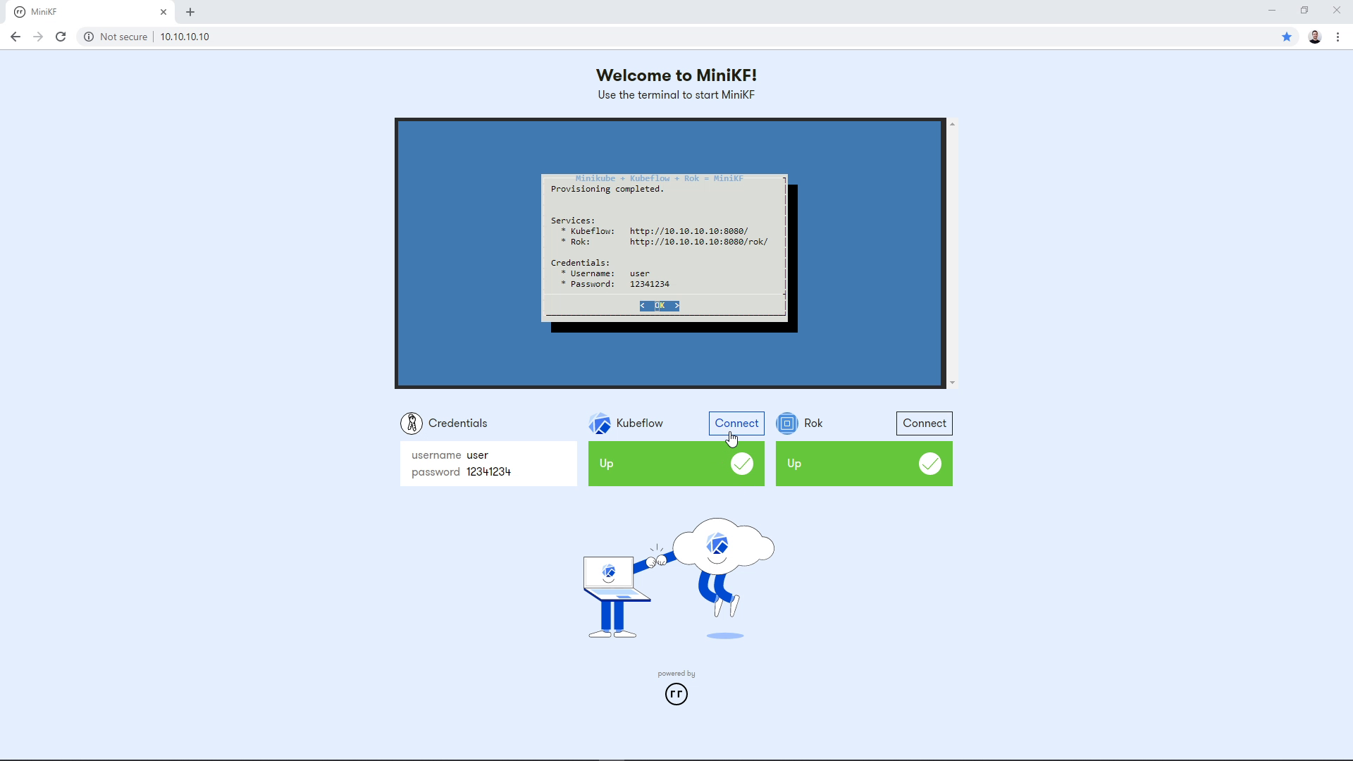
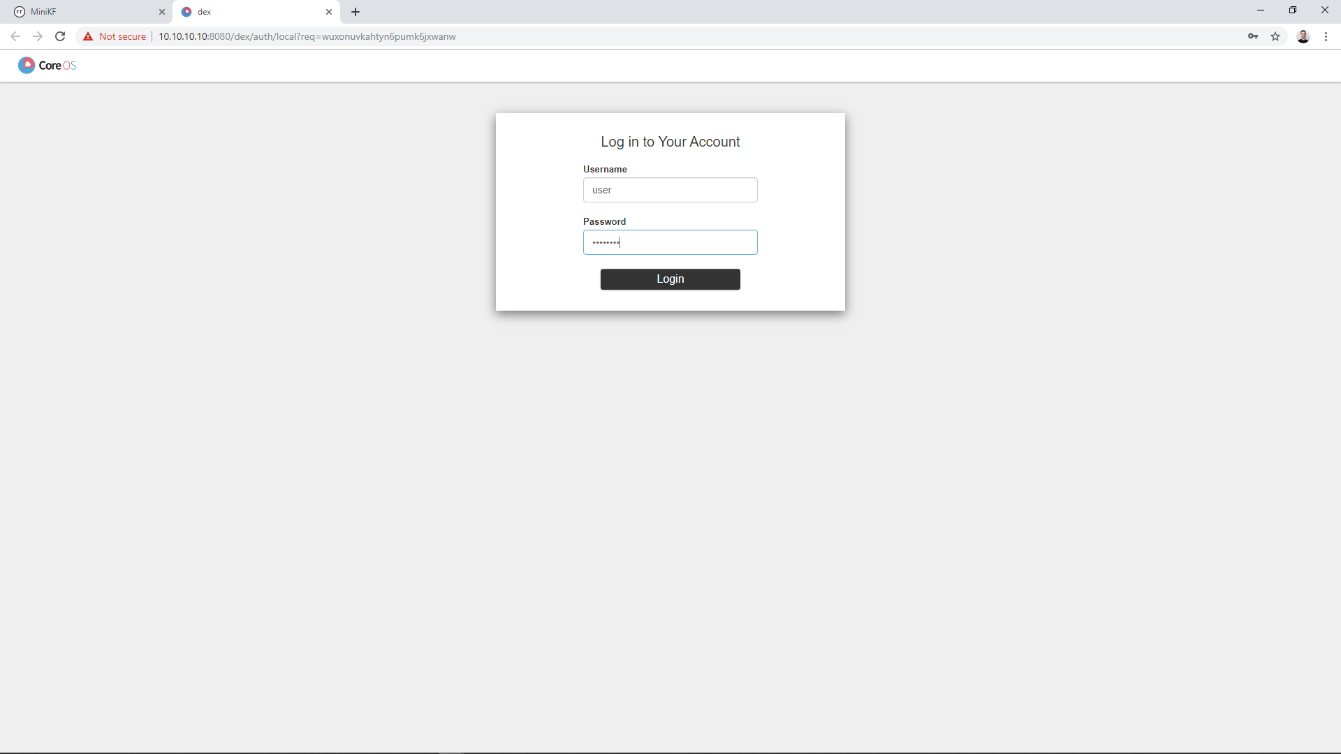
Log in using the credentials you see on your screen.
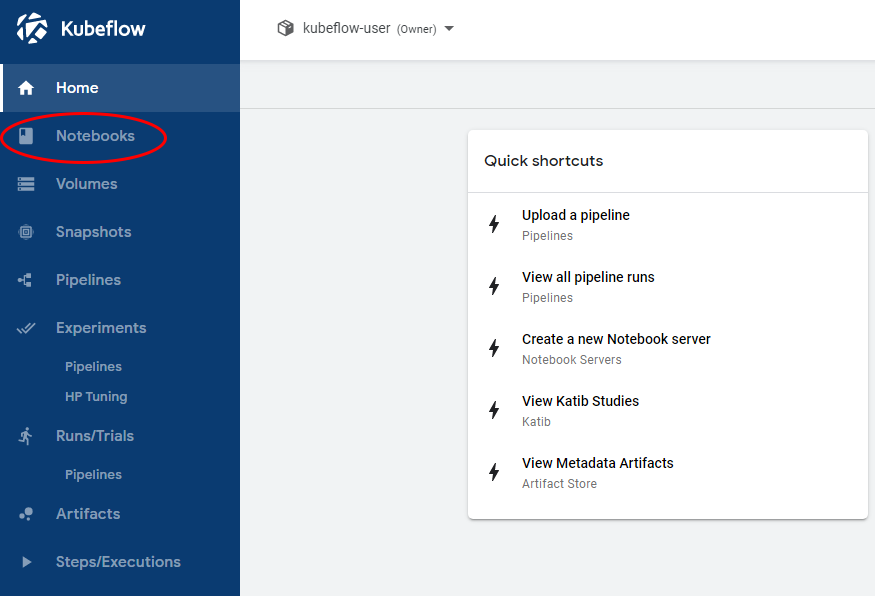
Once at Kubeflow’s Dashboard, click on the “Notebooks” link on the left pane to go to the Notebook Manager UI:
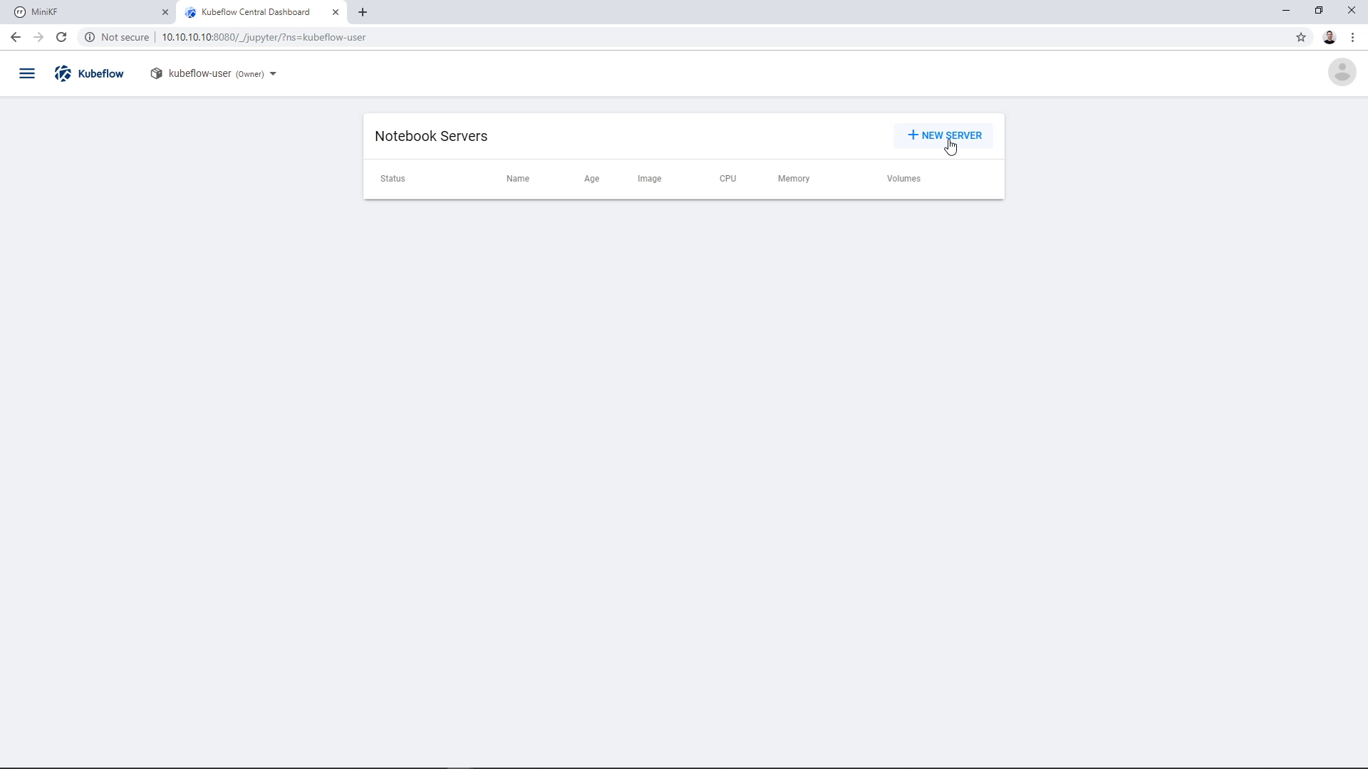
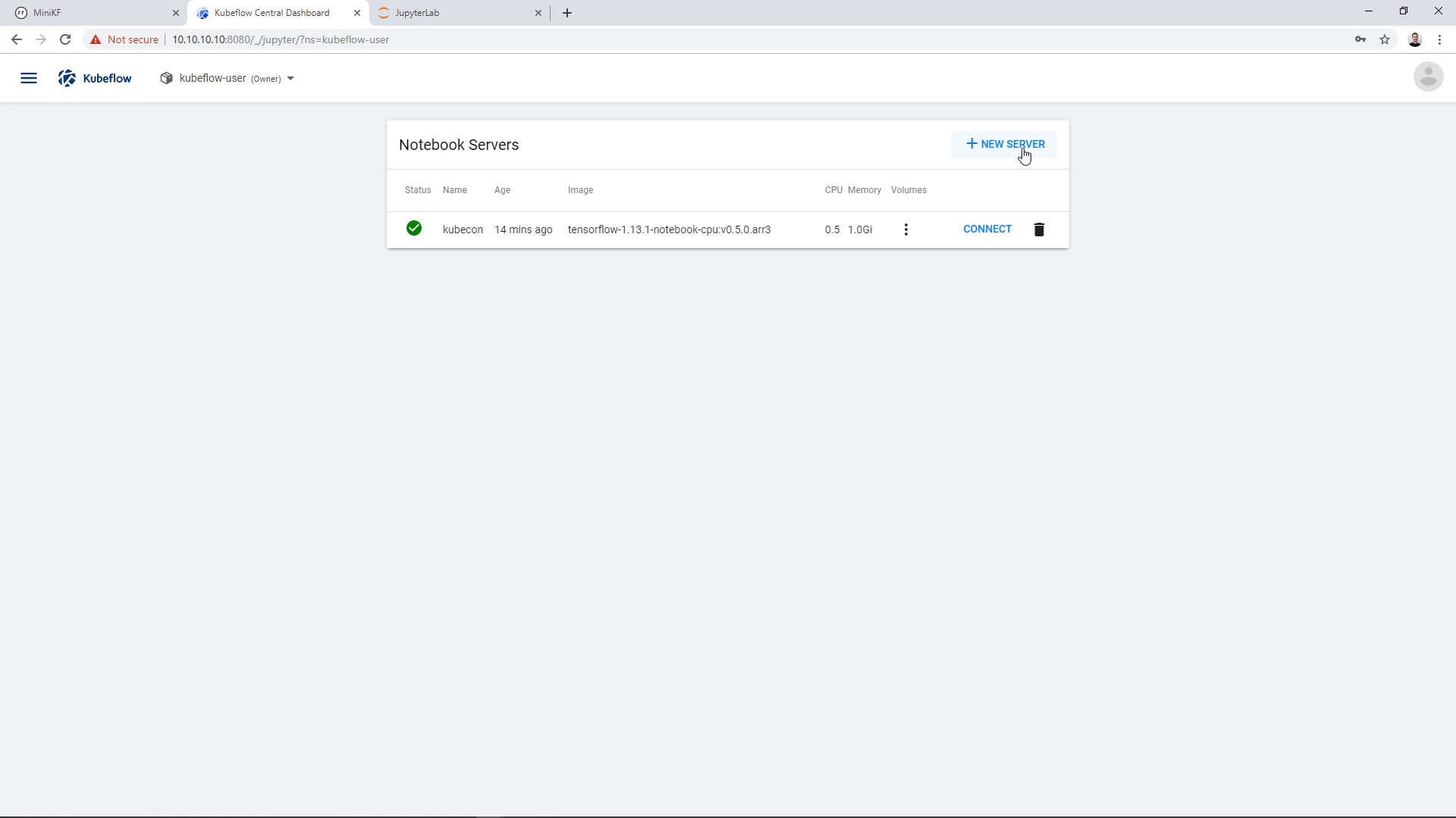
You are now at the Kubeflow Notebook Manager, showing the list of Notebook Servers, which is currently empty. Click on “New Server” to create a new Notebook Server:
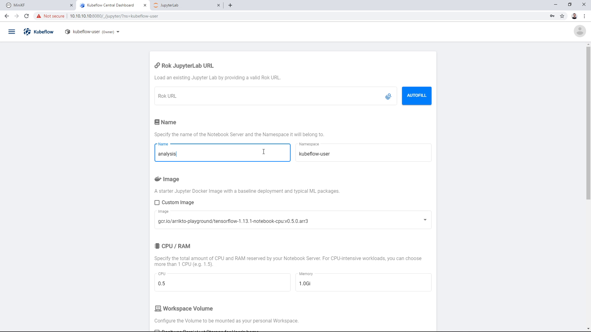
Enter a name for your new Notebook Server, and select Image, CPU, and RAM.
Make sure you have selected the following Docker image:
gcr.io/arrikto/jupyter-kale:v0.5.0-47-g2427cc9
Note that the image tag may differ.
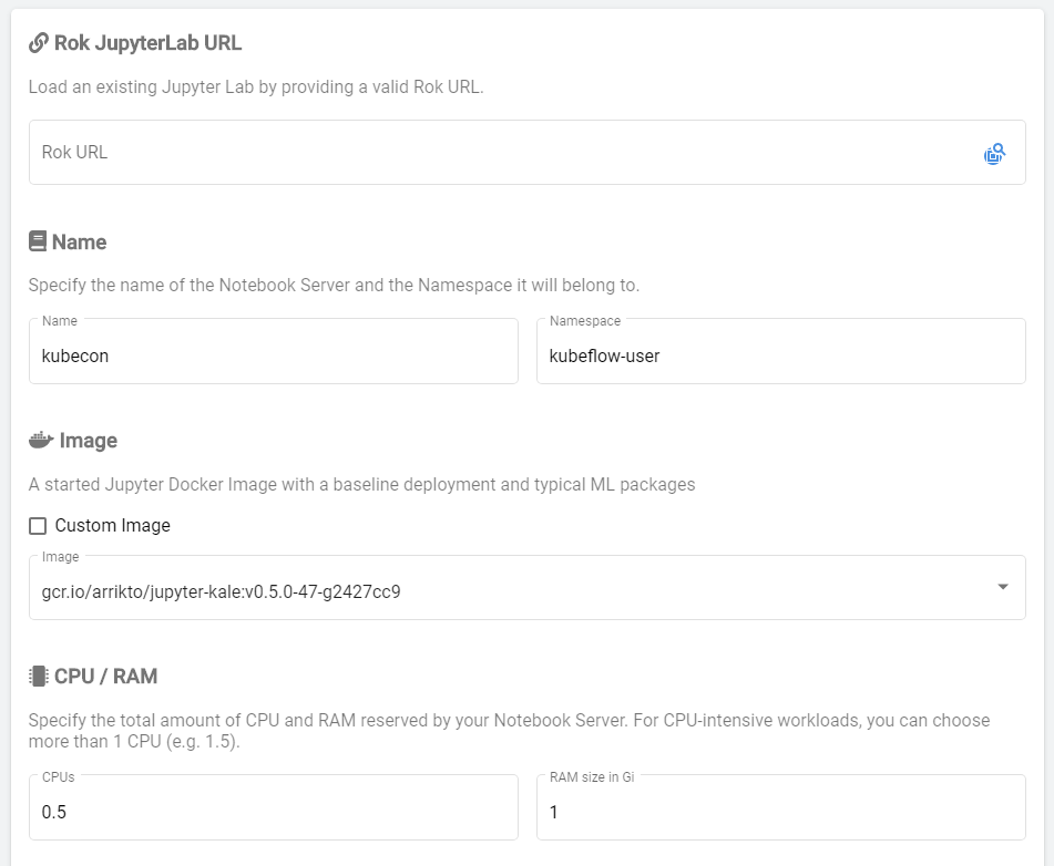
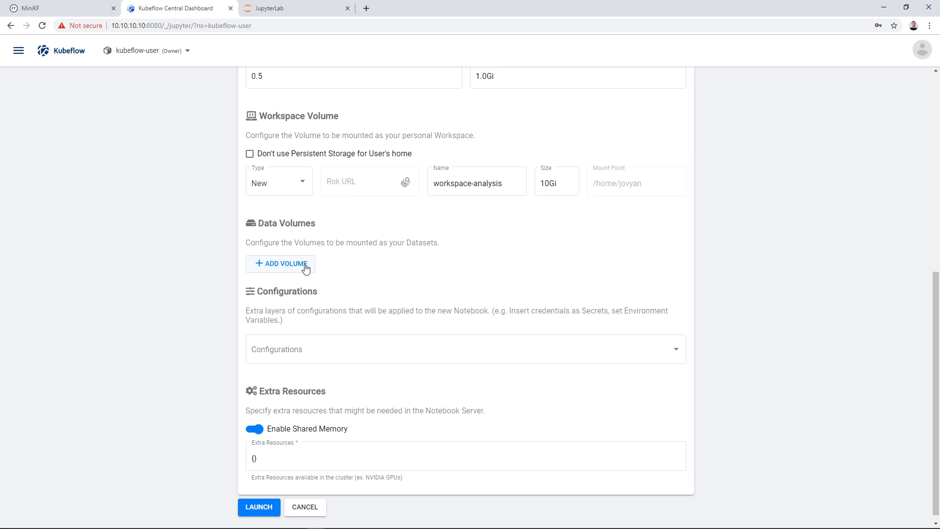
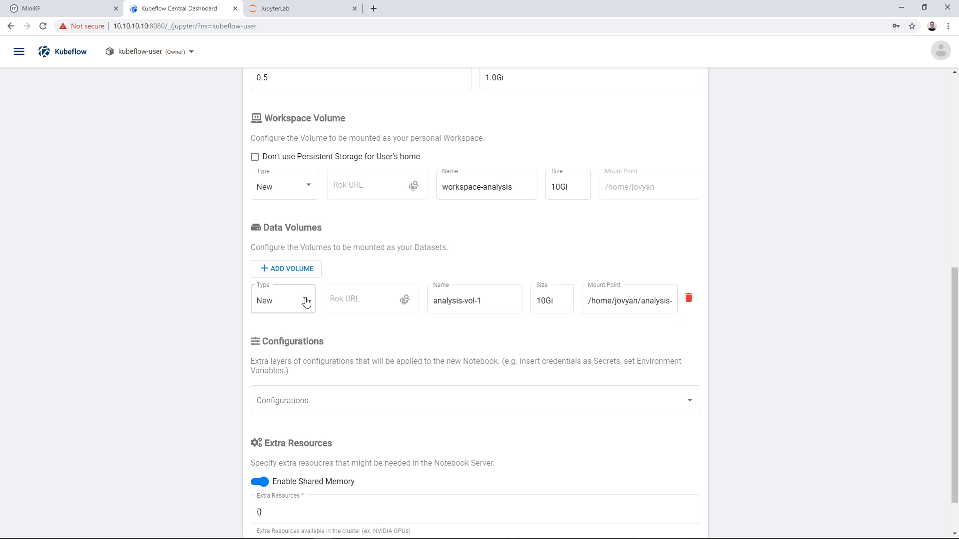
Add a new, empty Data Volume, for example of size 2GB, and name it “data” (you can give it any name you like, but then you will have to modify some commands in later steps):
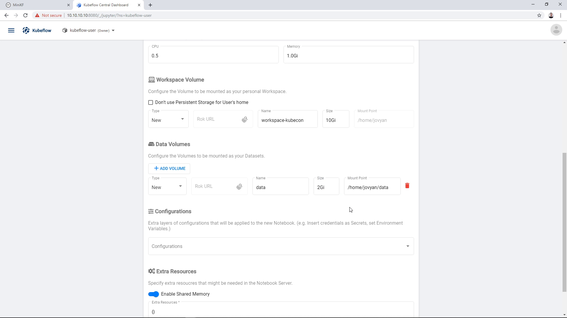
Once you select all options, click “Launch” to create the Notebook Server, and wait for it to get ready:
Once the Server is ready, the “Connect” button will become active (blue color). Click the “Connect” button to connect to your new Notebook Server:

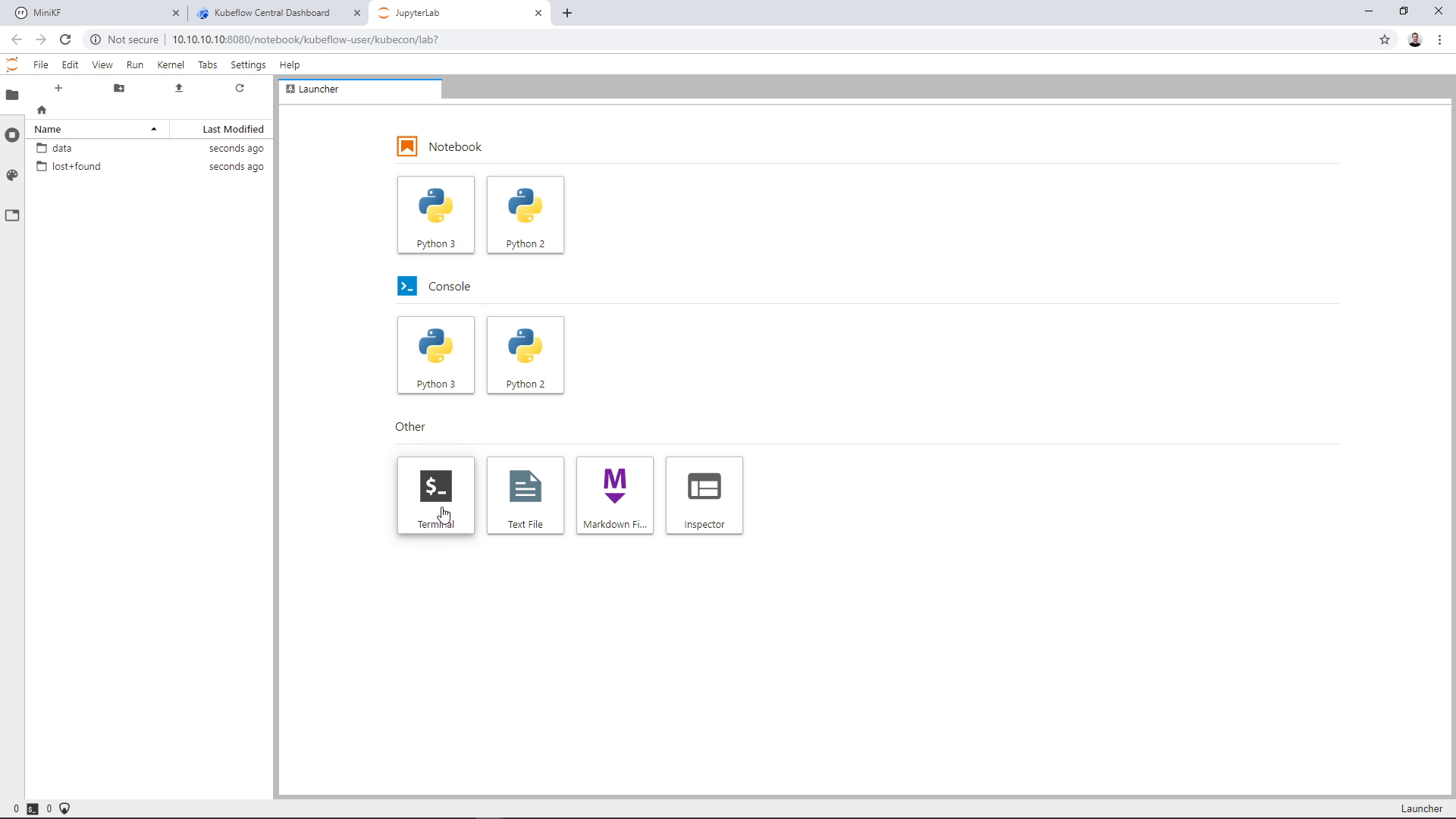
A new tab will open up with the JupyterLab landing page:
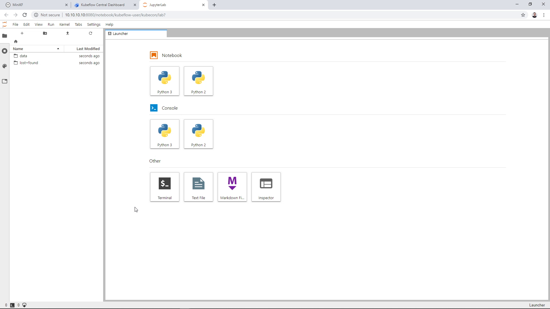
Bring in the Pipelines code and data
Create a new terminal in JupyterLab:
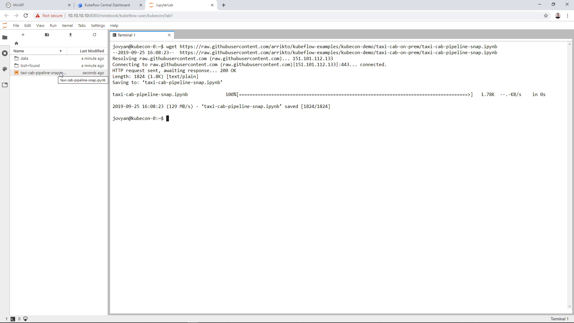
Bring in a pre-filled Notebook to run all the necessary commands:
wget https://raw.githubusercontent.com/arrikto/kubeflow-examples/kubecon-demo/taxi-cab-on-prem/taxi-cab-pipeline-snap.ipynb
The Notebook will appear on the left pane of your JupyterLab:
Double-click the notebook file to open it and run the cells one-by-one:
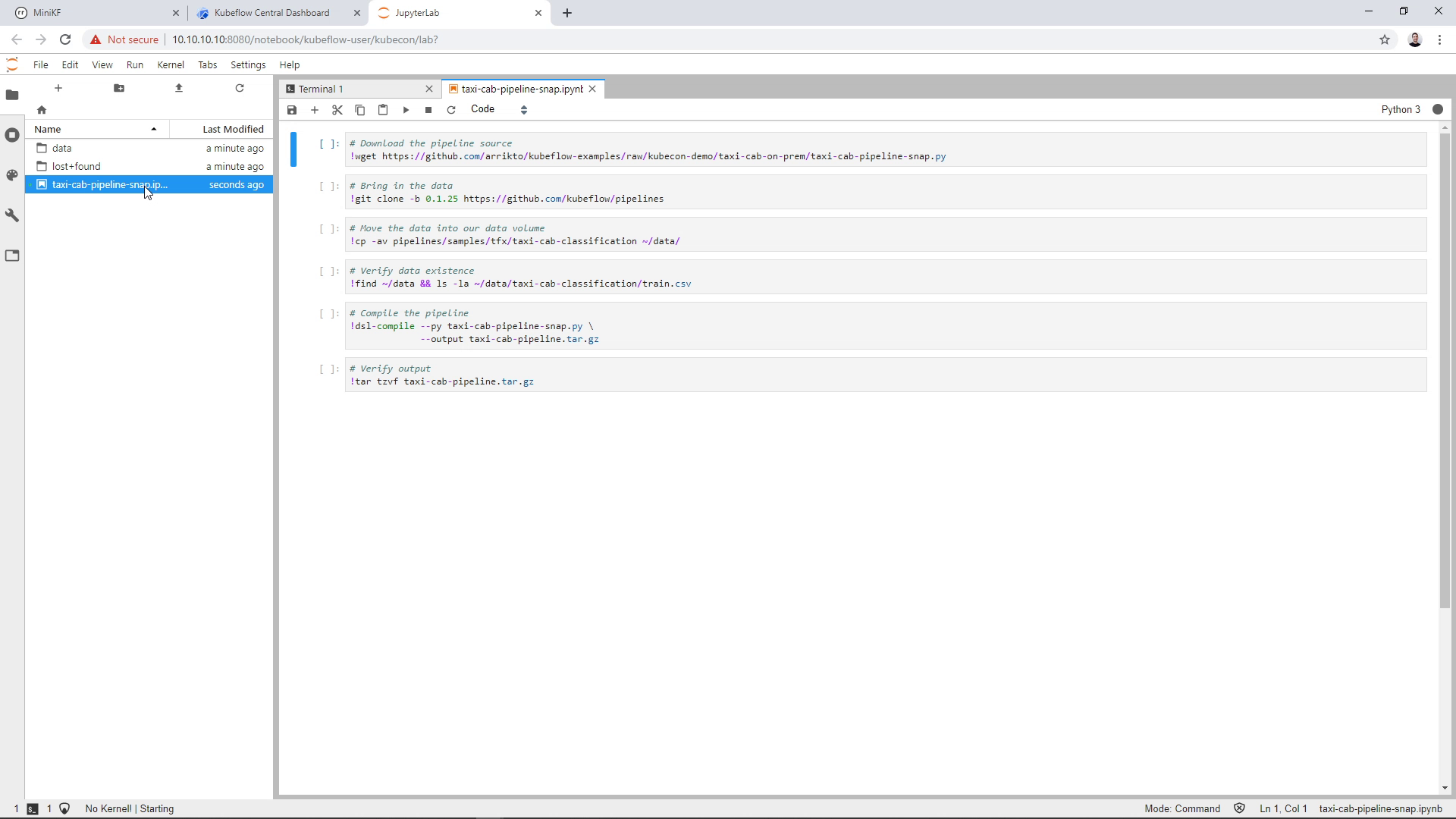
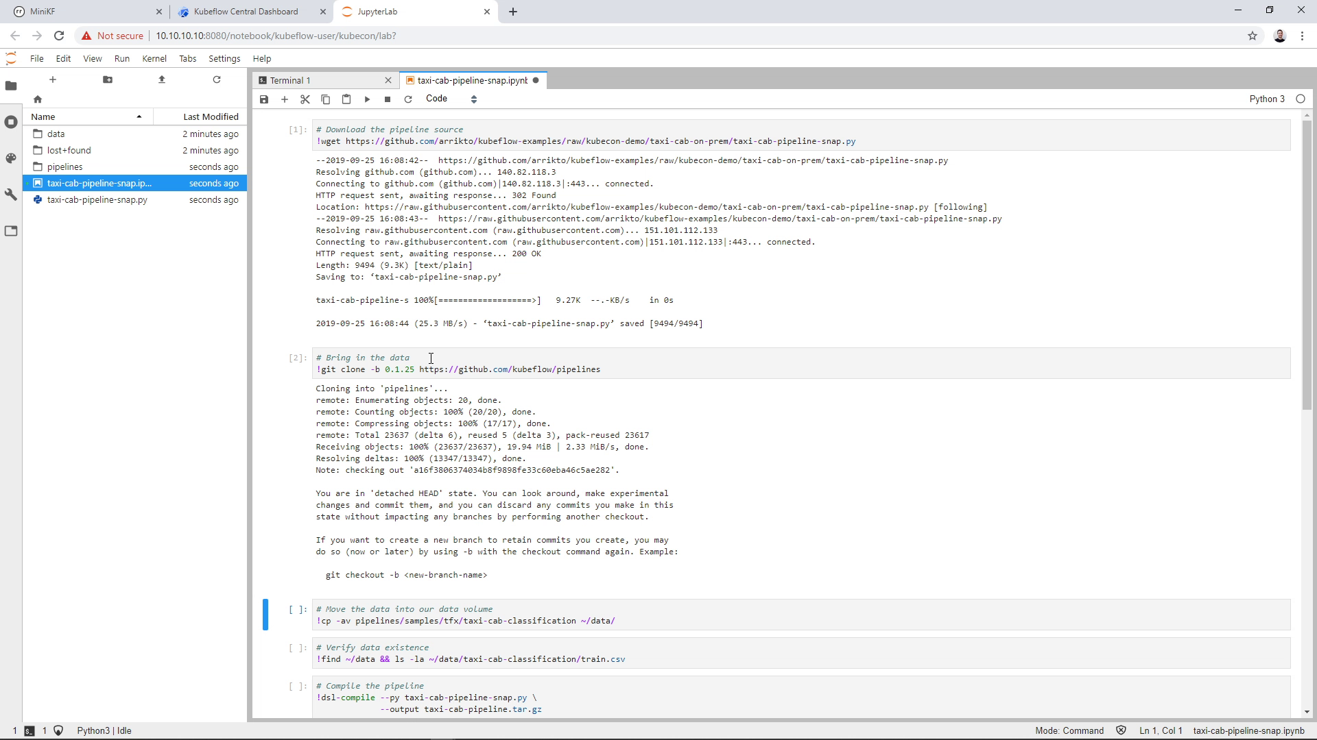
Run the first cell to download the Arrikto’s pipeline code to run the Chicago Taxi Cab example on-prem:
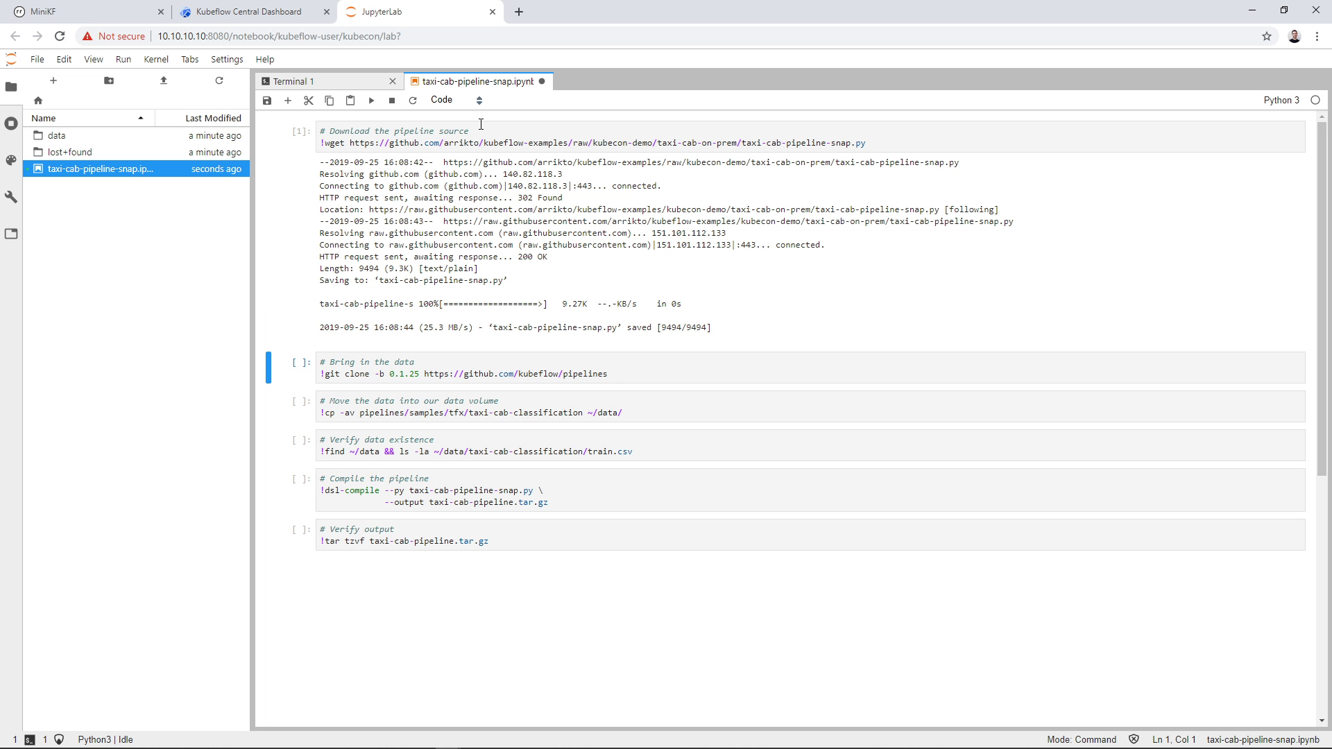
Run the second cell to ingest the data:
Run the third cell to move the ingested data to the Data Volume of the Notebook. (Note that if you didn’t name your Data Volume “data”, then you have to slightly modify this command):
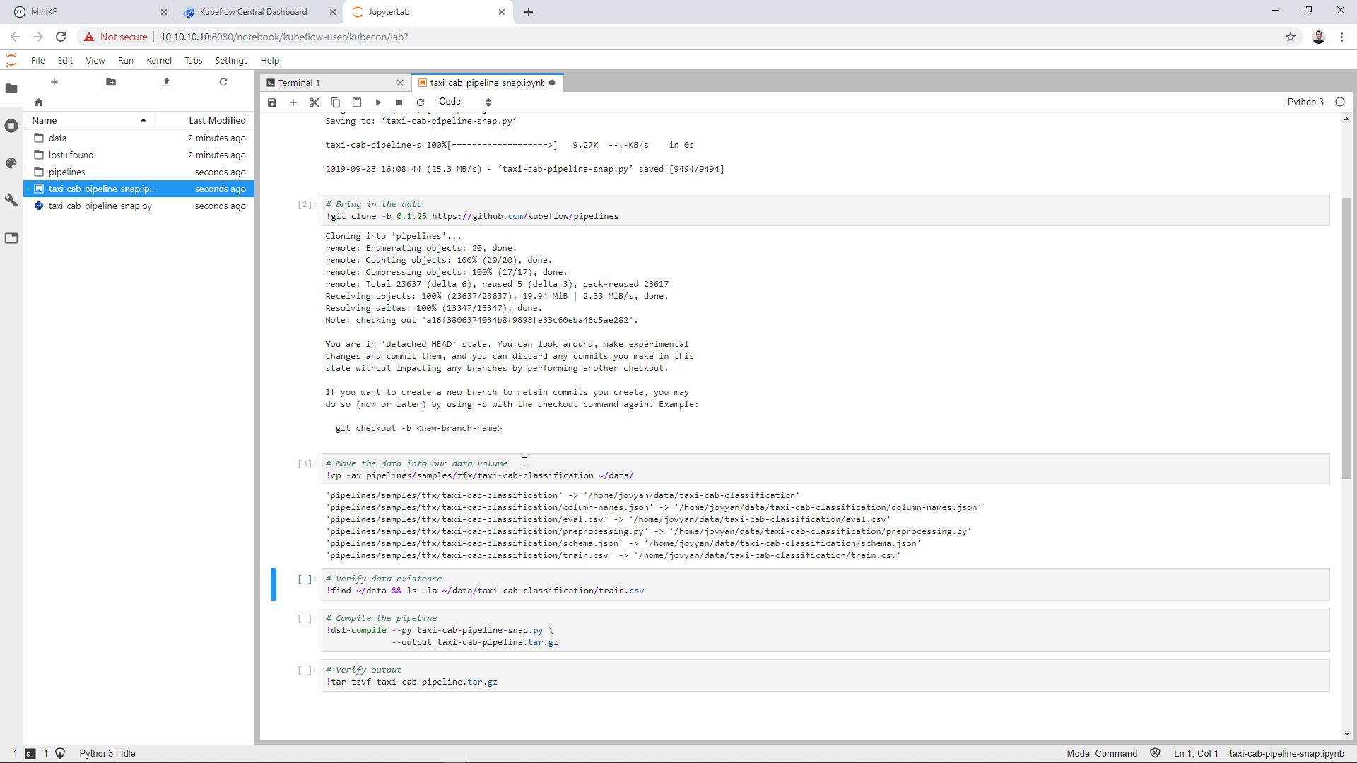
Run the fourth cell to verify that data exist inside the Data Volume. Note that you should have the taxi-cab-classification directory under the data directory, not just the files. You now have a local Data Volume populated with the data the pipeline code needs (if you didn’t give the name “data” to your Data Volume, then you have to make sure that your Data Volume has these files in it):
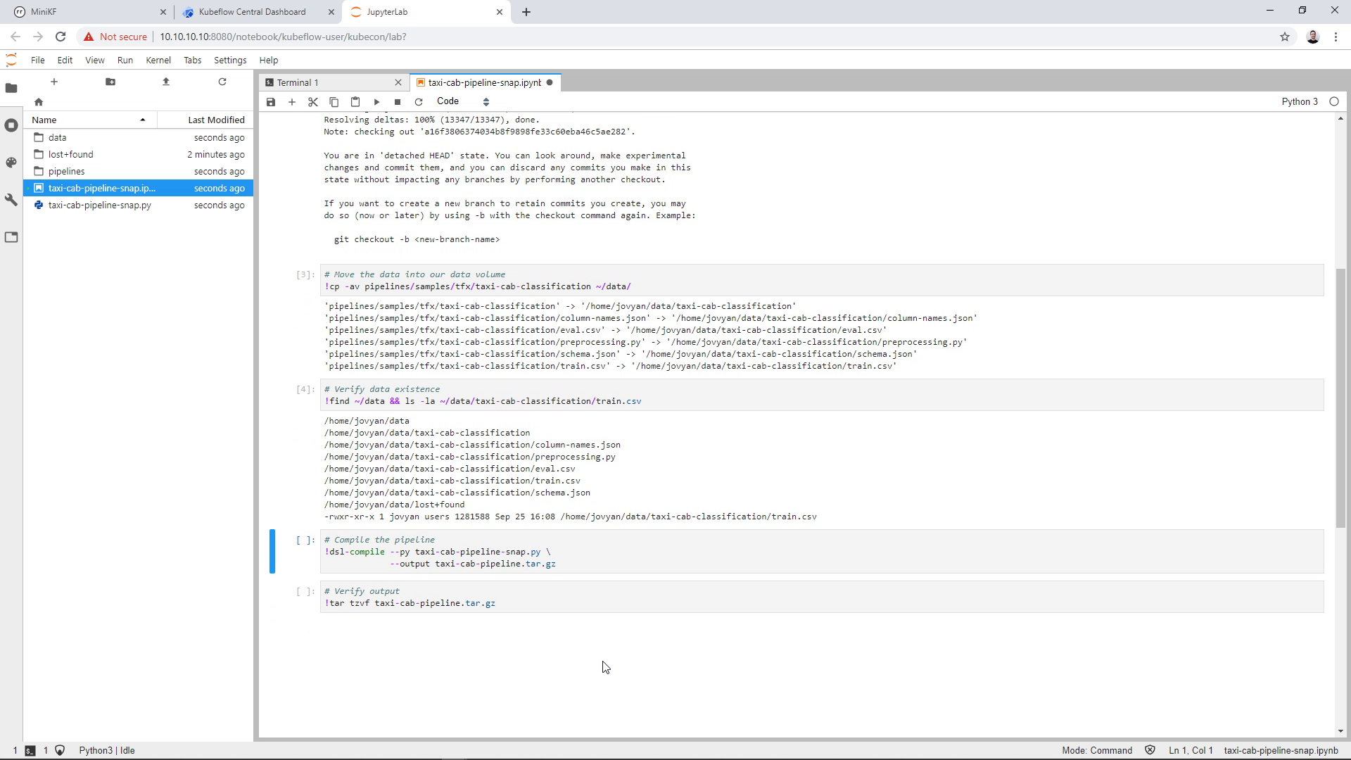
Run the fifth cell to compile the pipeline source code:
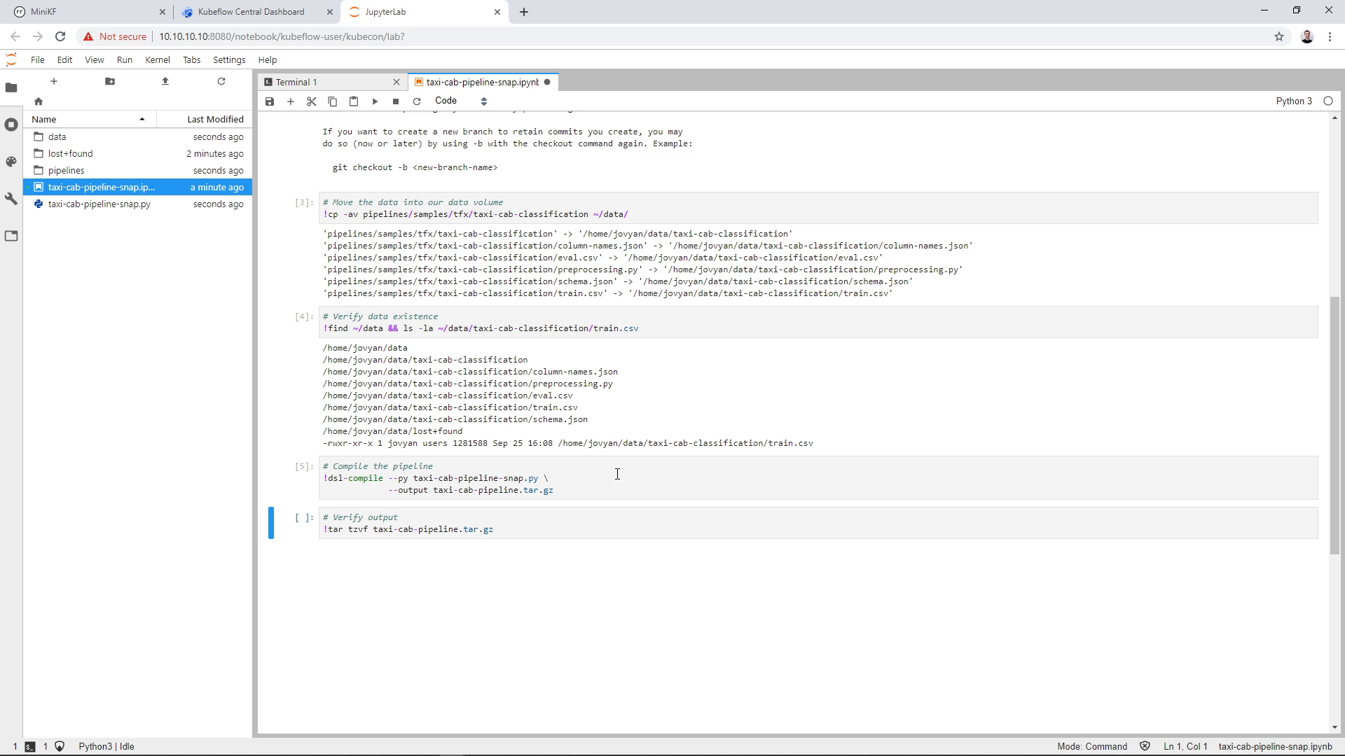
Run the sixth cell to verify the output of the compiled pipeline:
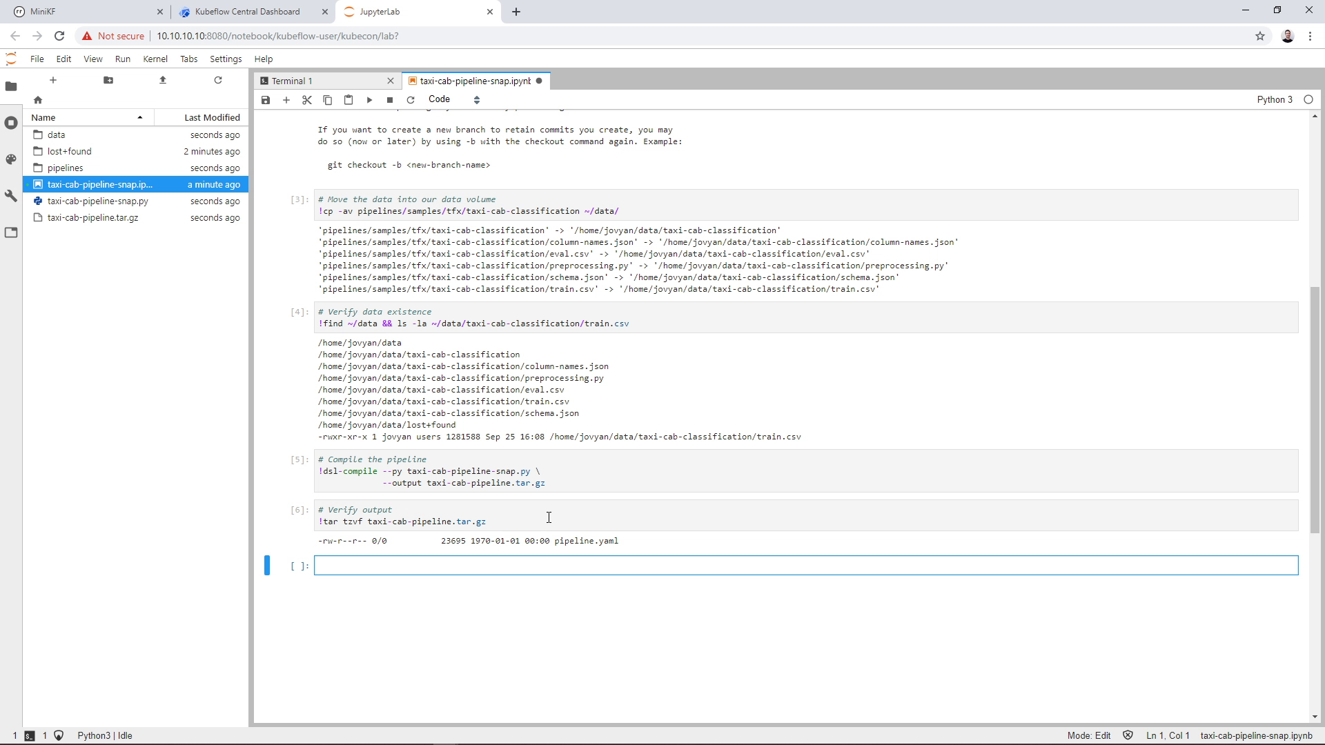
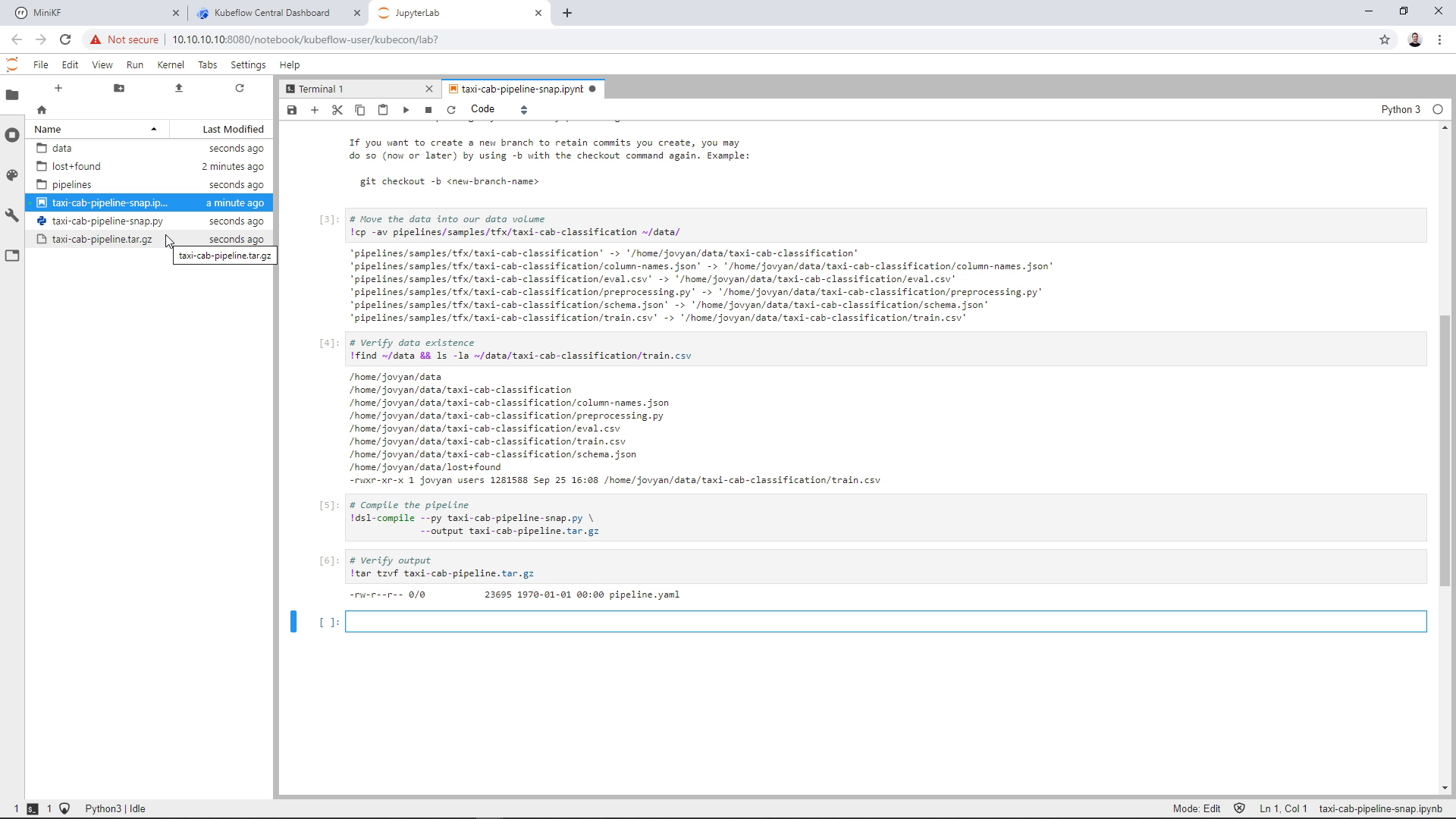
The file containing the compiled pipeline appears on the left pane of your JupyterLab:
Snapshot the Data Volume
In later steps, the pipeline is going to need the data that we brought into the Data Volume previously. For this reason, we need a snapshot of the Data Volume. As a best practice, we will snapshot the whole JupyterLab, and not just the Data Volume, in case the user wants to go back and reproduce their work.
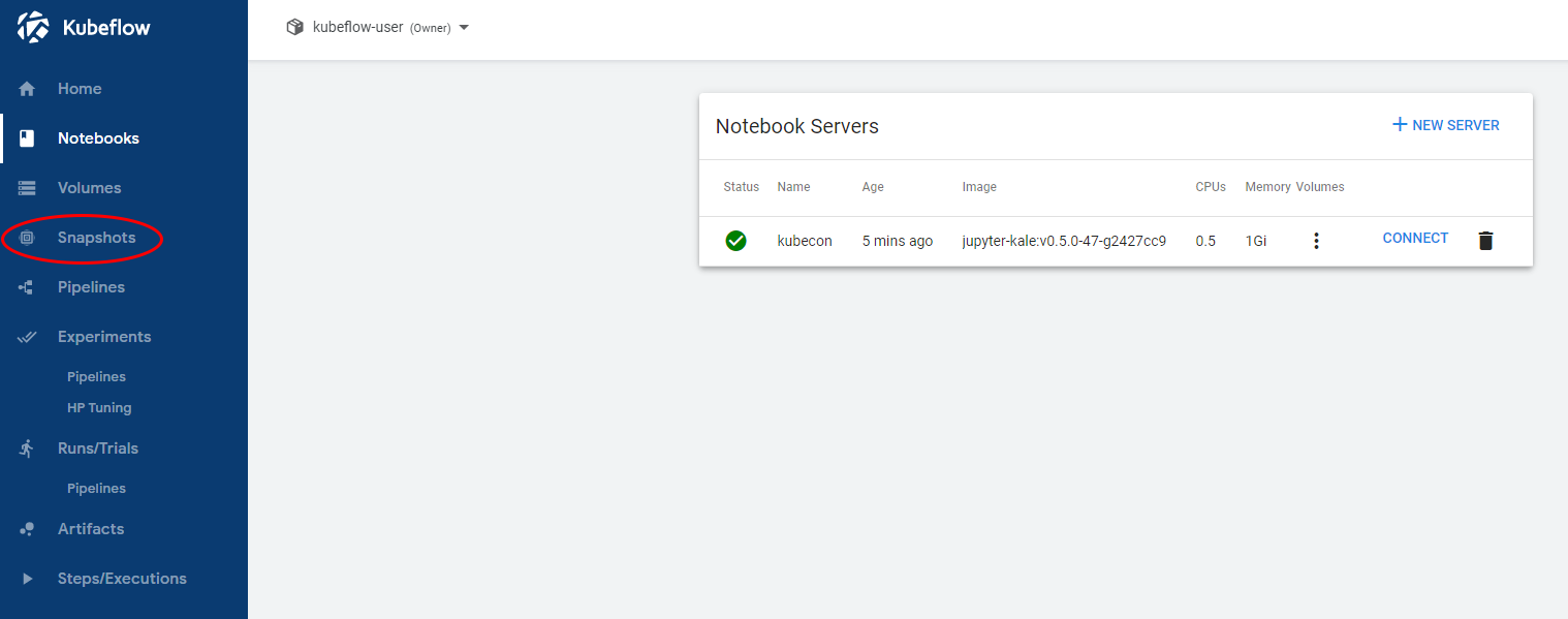
We will use Rok, which is already included in MiniKF, to snapshot the JupyterLab. On the Kubeflow left pane, click on the “Snapshots” link to go to the Rok UI. Alternatively, you can go to the MiniKF landing page and click the “Connect” button next to Rok:
This is the Rok UI landing page:
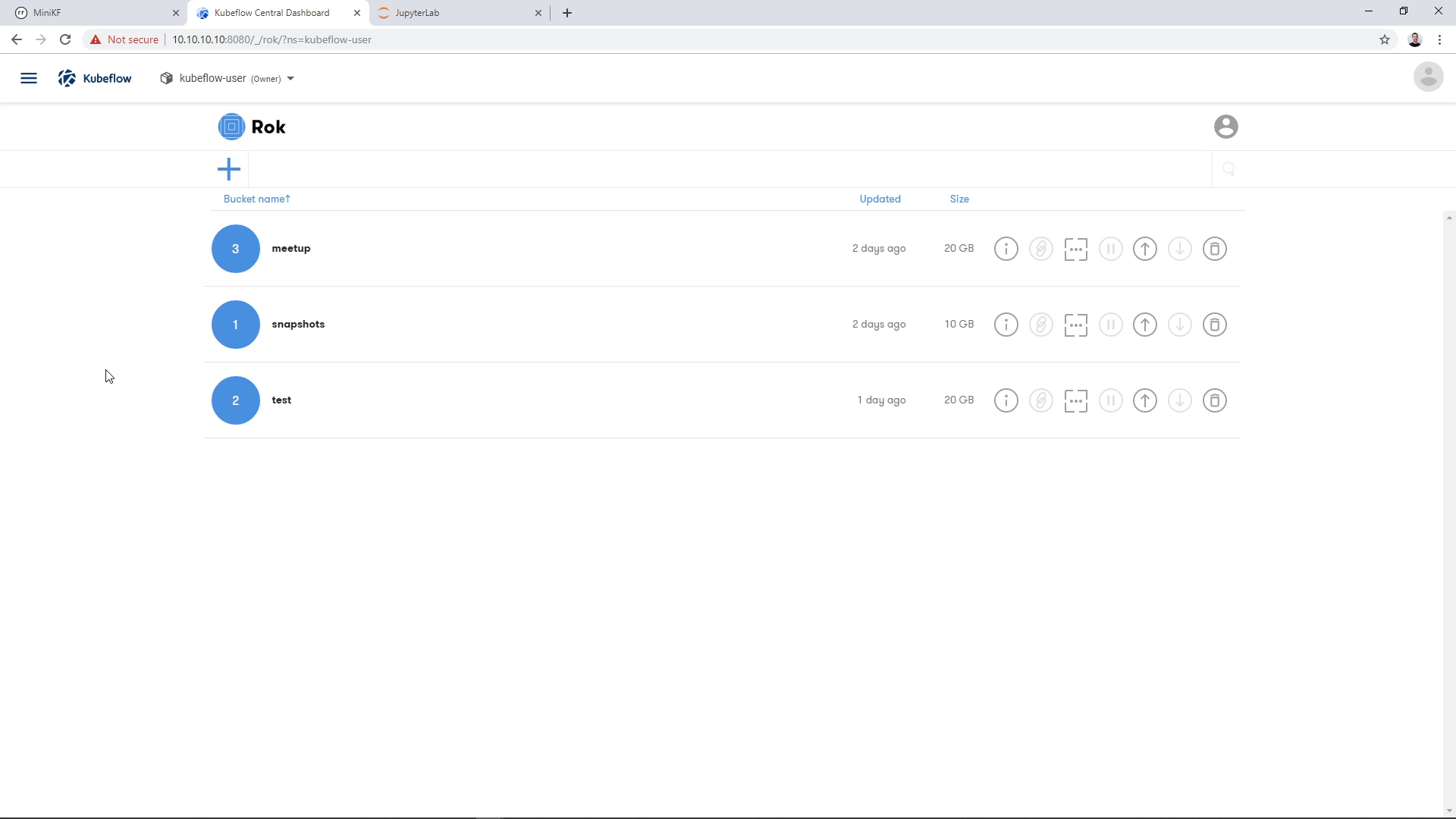
Create a new bucket to host the new snapshot. Click on the “+” button on the top left:
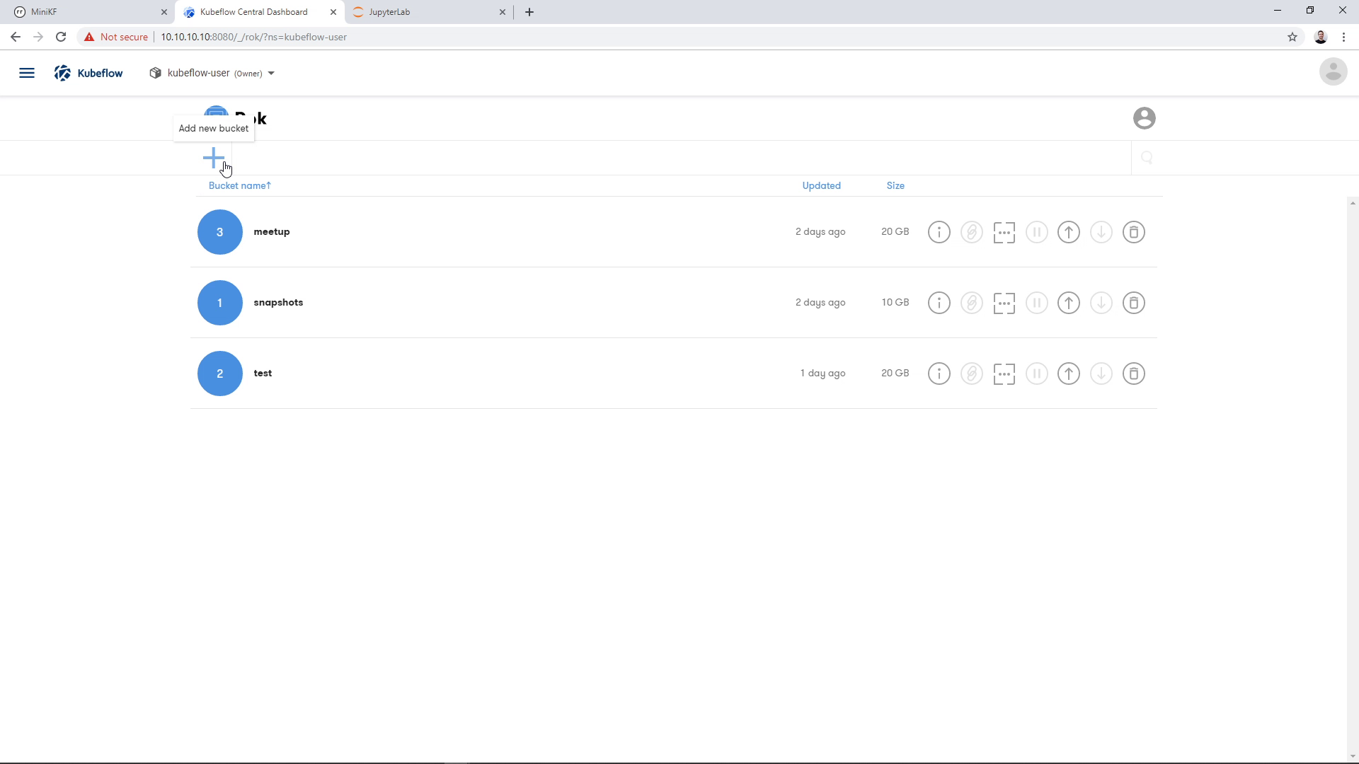
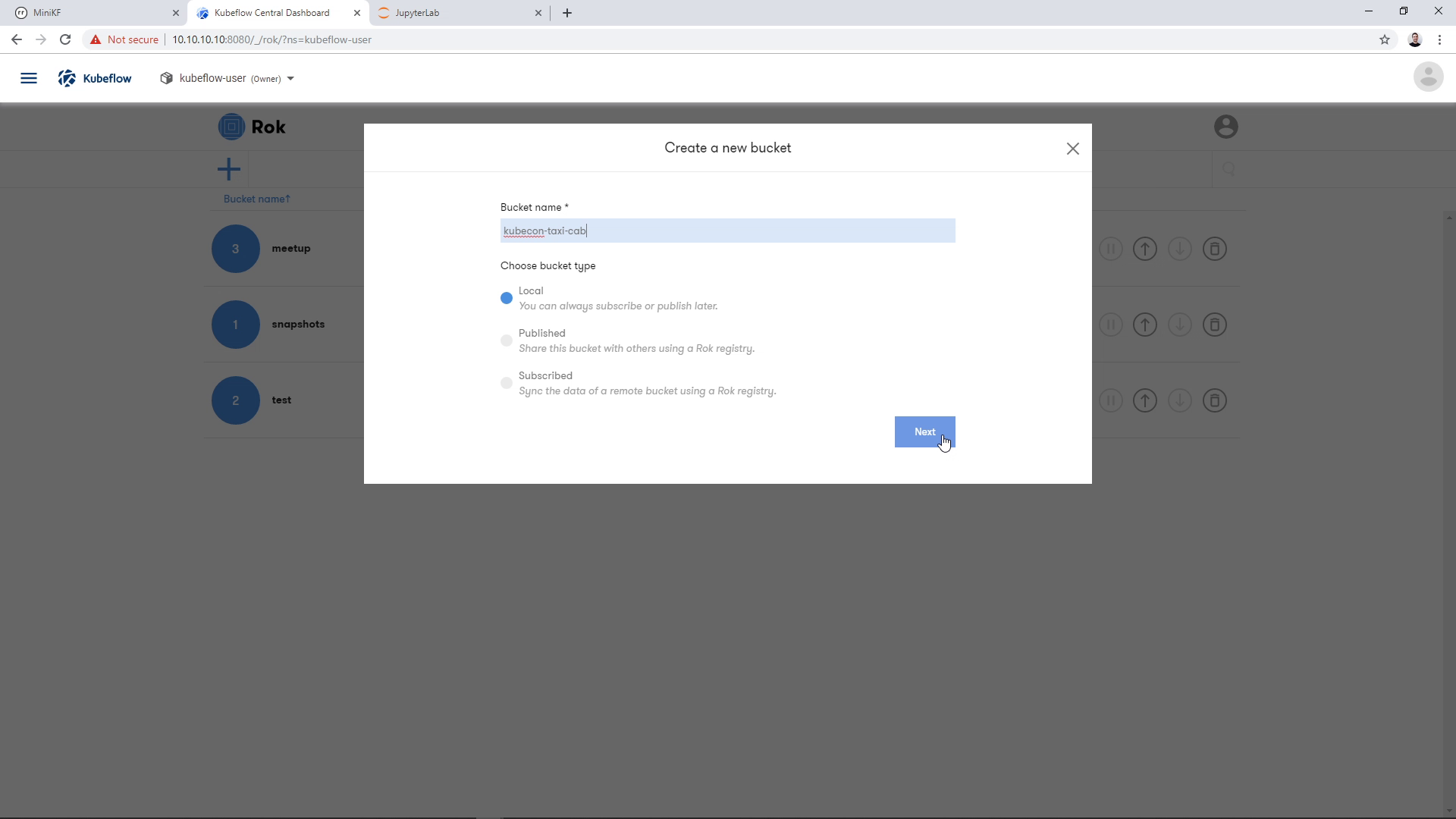
A dialog will appear asking for a bucket name. Give it a name and click “Next”. We will keep the bucket “Local” for this demo:
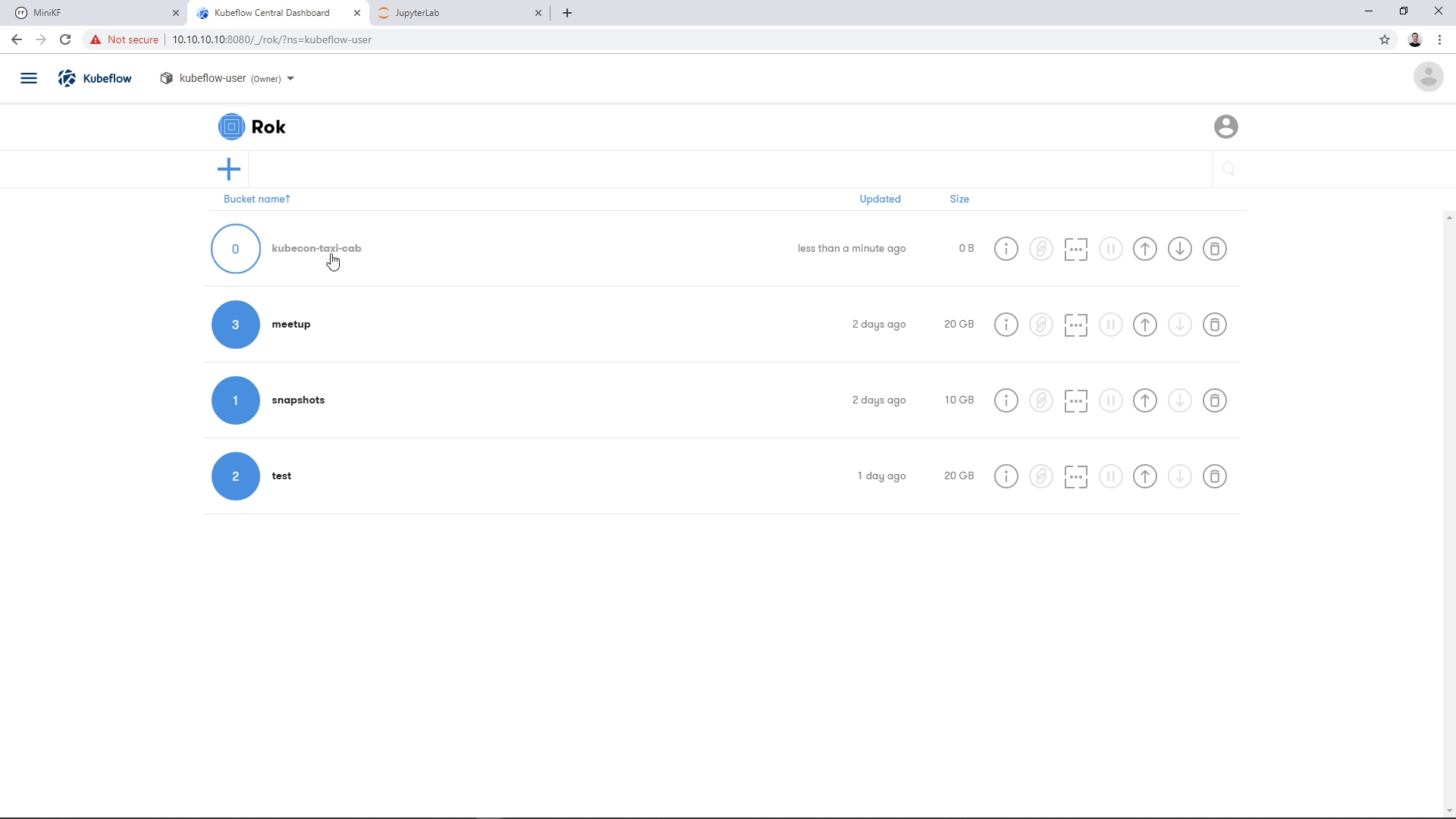
Clicking “Next” will result in a new, empty bucket appearing in the landing page. Click on the bucket, to go inside:
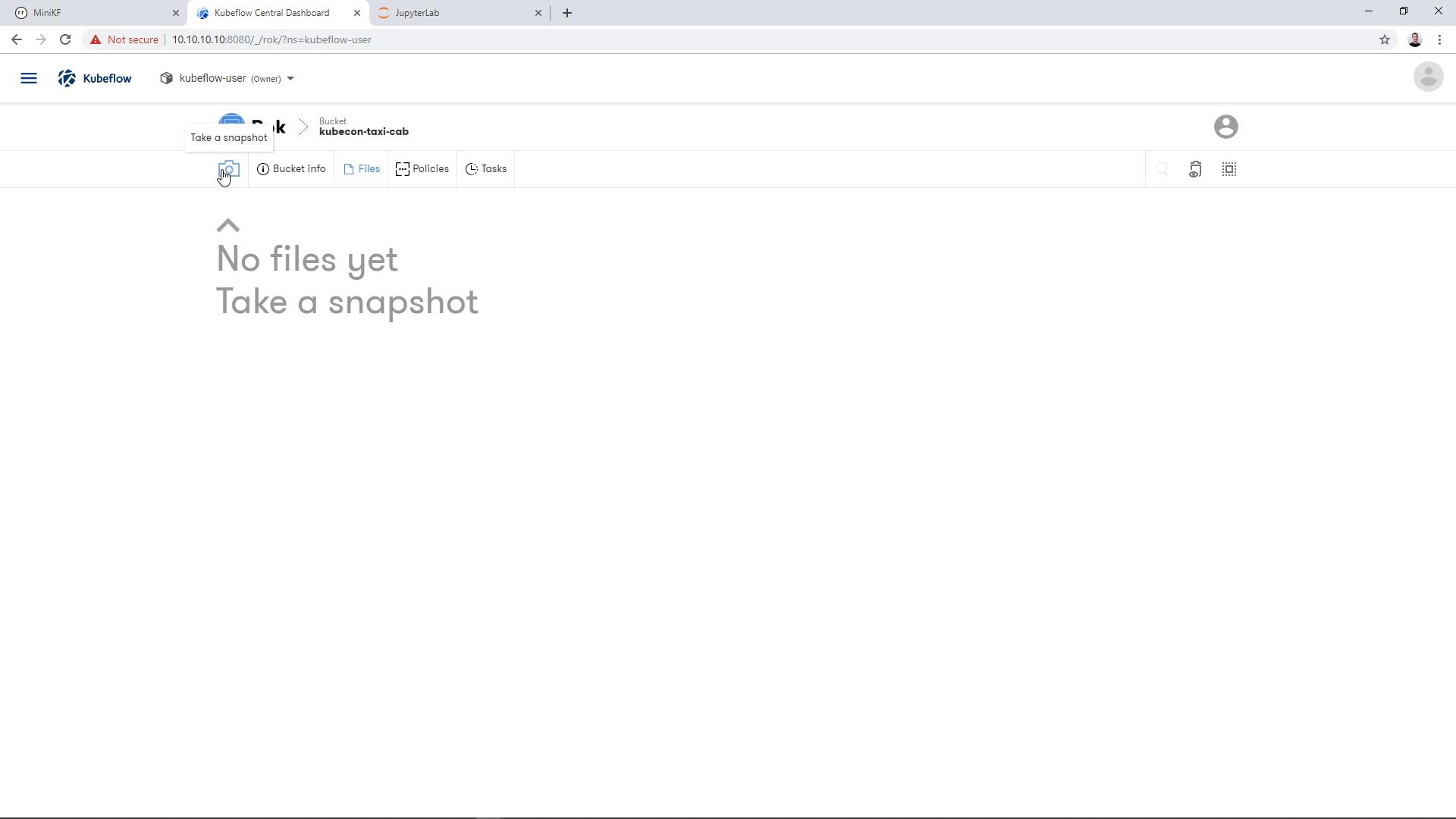
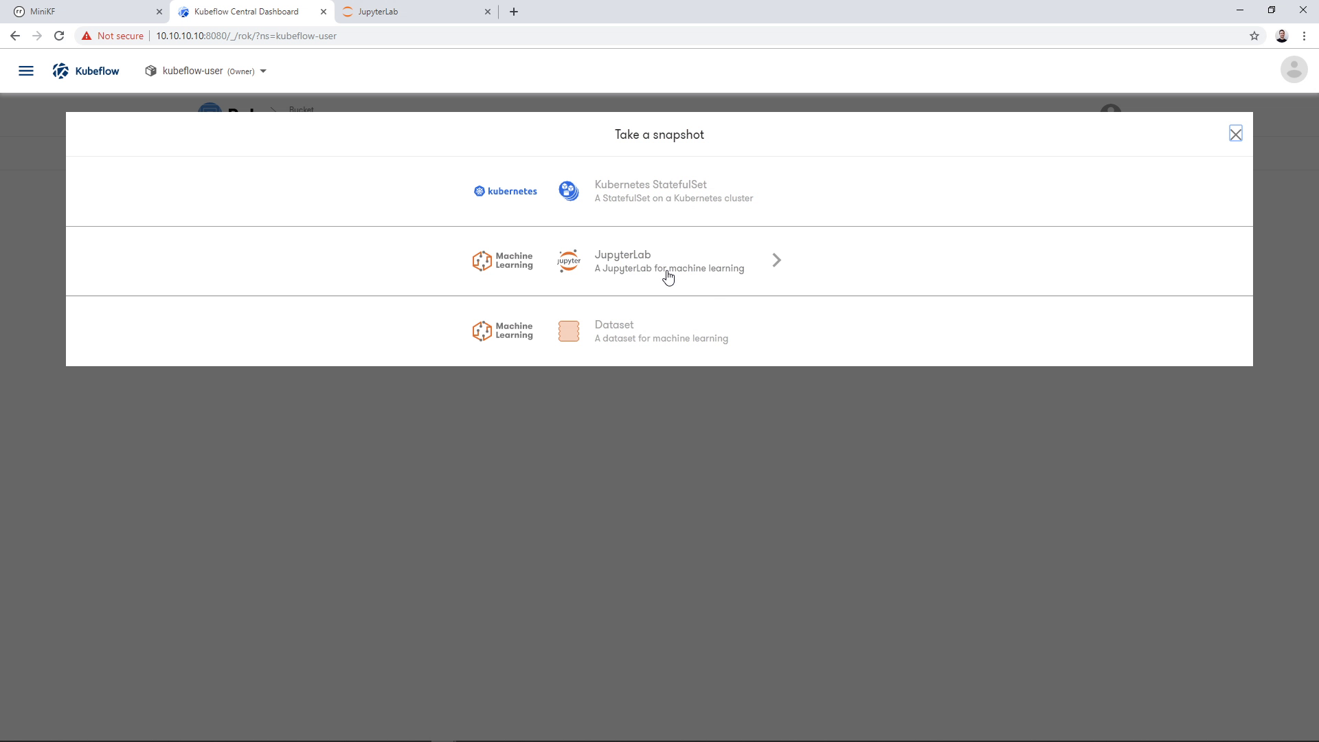
Once inside the bucket, click on the Camera button to take a new snapshot:
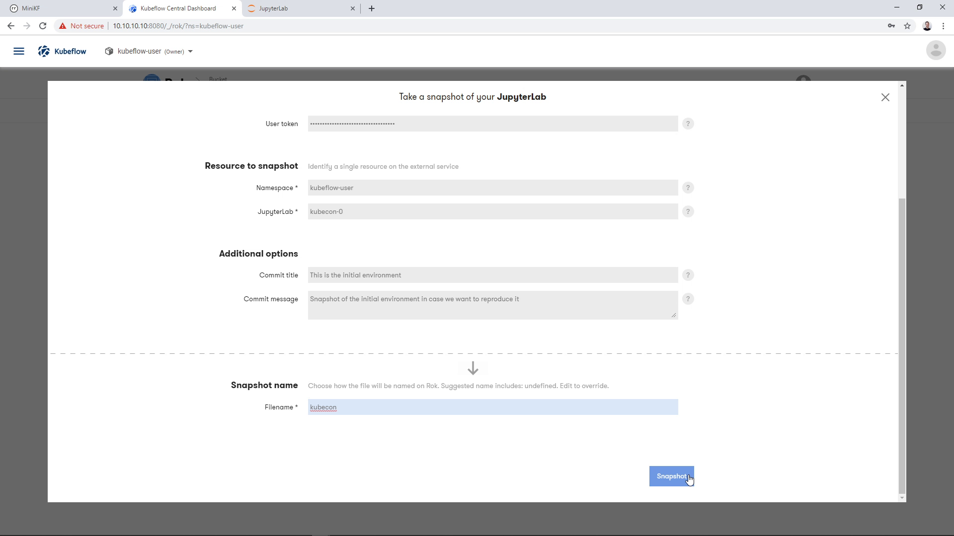
By clicking the Camera button, a dialog appears asking for the K8s resource that we want to snapshot. Choose the whole “JupyterLab” option, not just the single Data Volume (“Dataset”):
Most fields will be pre-filled with values automatically by Rok, for convenience. Select your JupyterLab from the dropdown list:
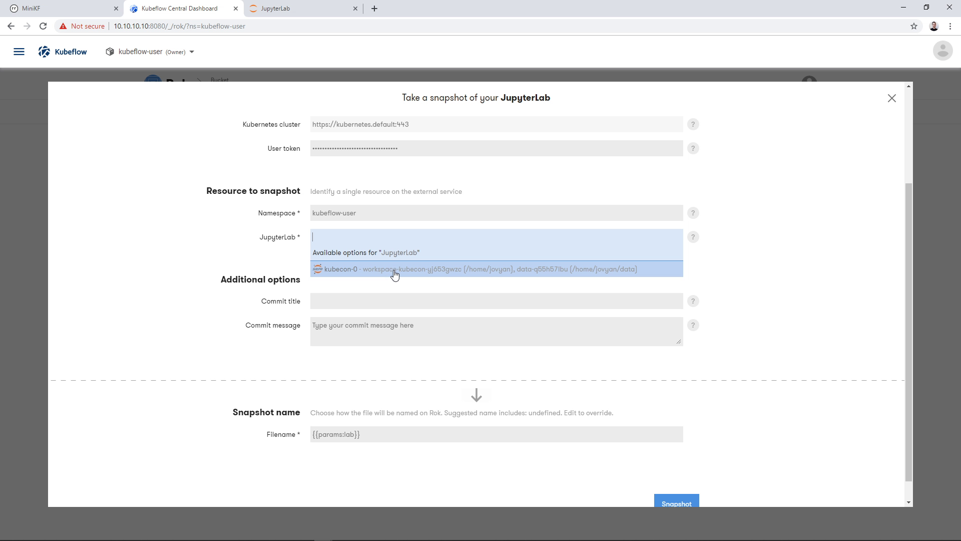
Provide a commit title and a commit message for this snapshot. This is to help you identify the snapshot version in the future, the same way you would do with your code commits in Git:
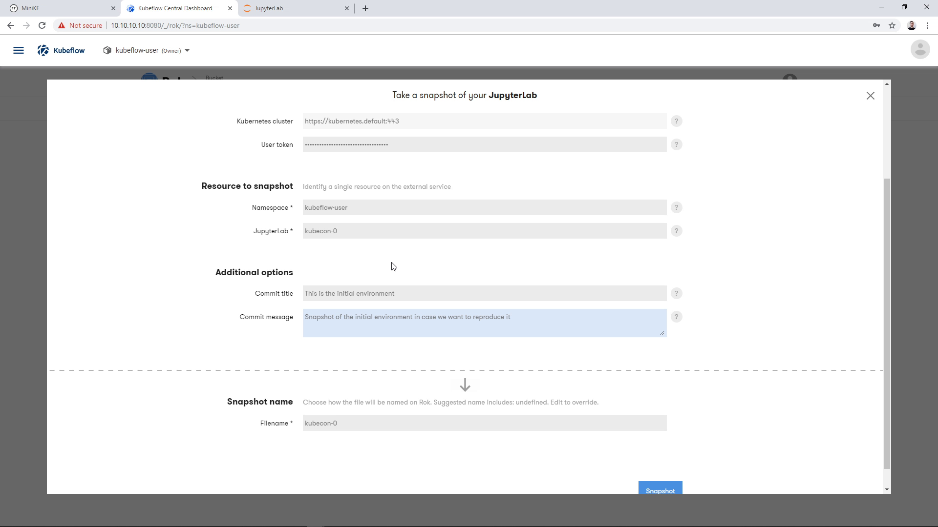
Then, choose a name for your snapshot:
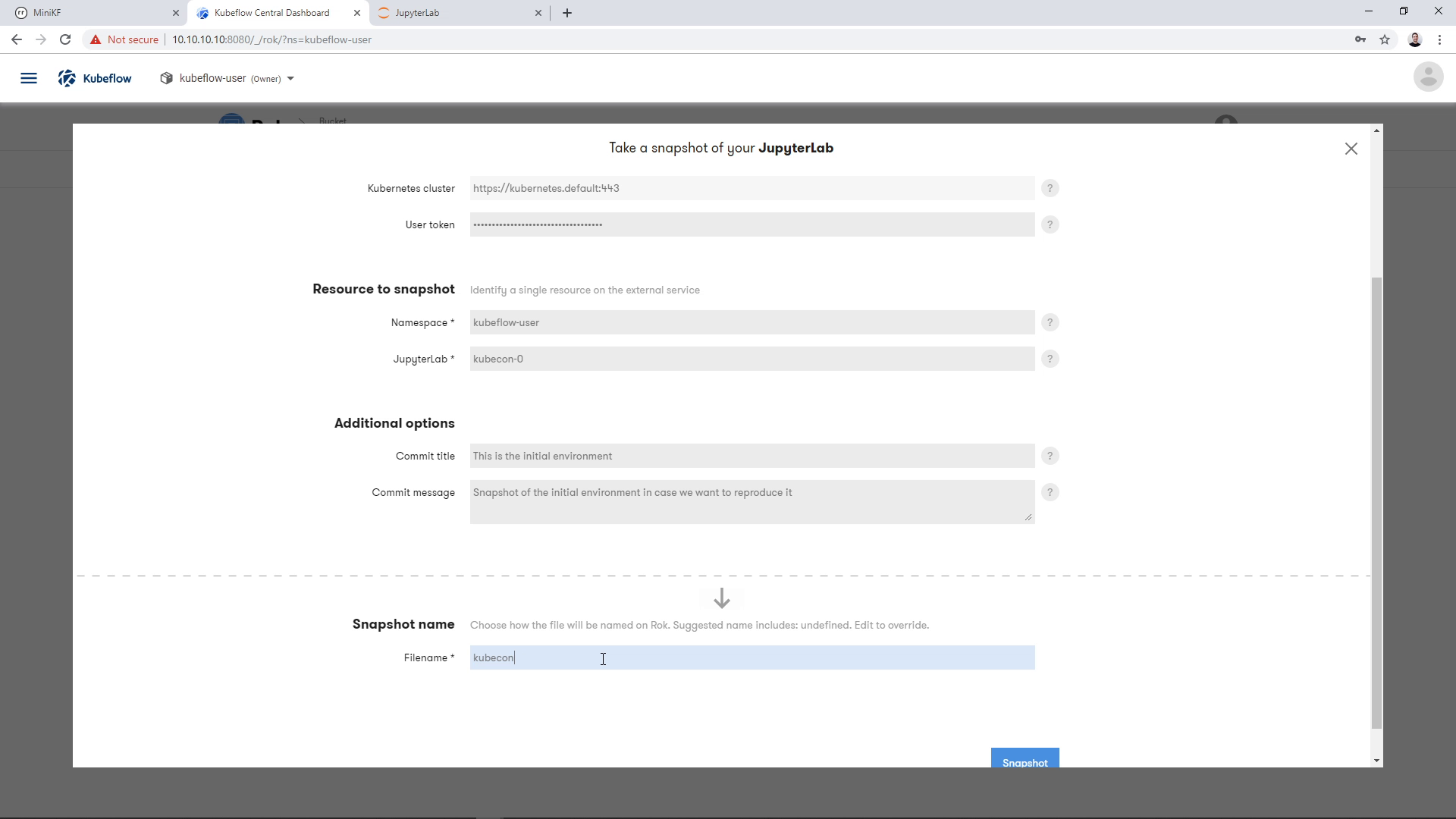
Take the snapshot, by clicking the “Snapshot” button:
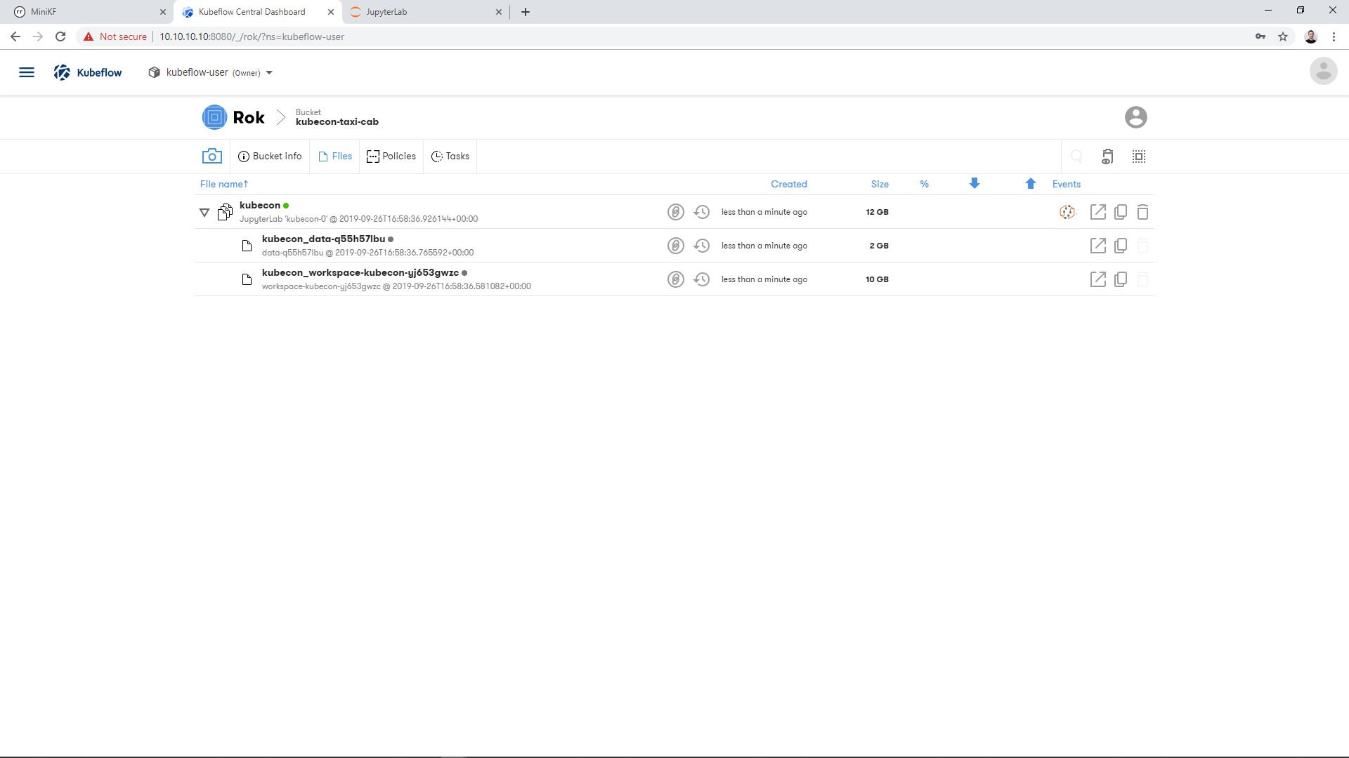
Once the operation completes, you will have a snapshot of your whole JupyterLab. This means you have a snapshot of the Workspace Volume and a snapshot of the Data Volume, along with all the corresponding JupyterLab metadata to recreate the environment with a single click. The snapshot appears as a file inside your new bucket. Expanding the file will let you see the snapshot of the Workspace Volume and the snapshot of the Data Volume:
Now that we have both the pipeline compiled and a snapshot of the Data Volume, let’s move on to run the pipeline and seed it with the data we prepared.
Upload the Pipeline to KFP
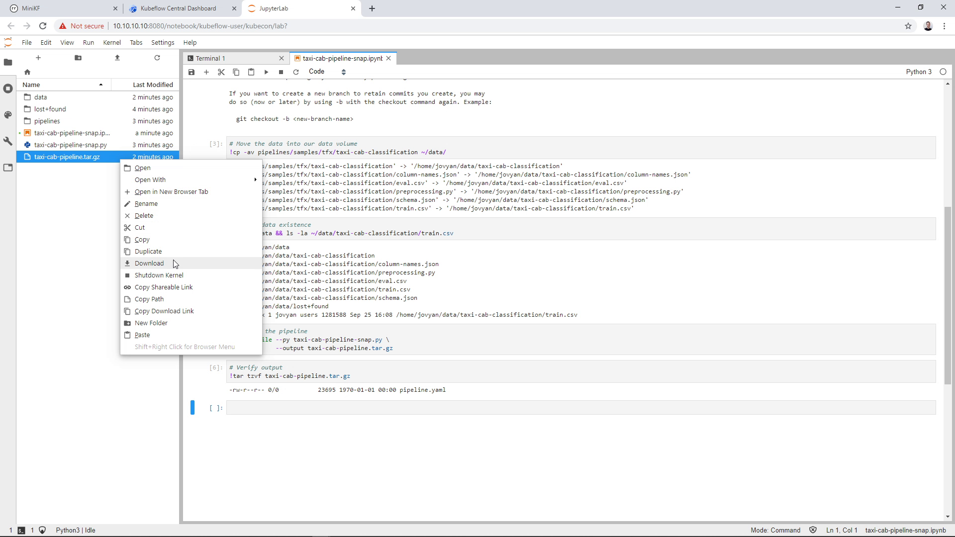
Before uploading the pipeline to KFP, we first need to download the compiled pipeline locally. Go back to your JupyterLab and download the compiled pipeline. To do so, right click on the file on JupyterLab’s left pane, and click “Download”:
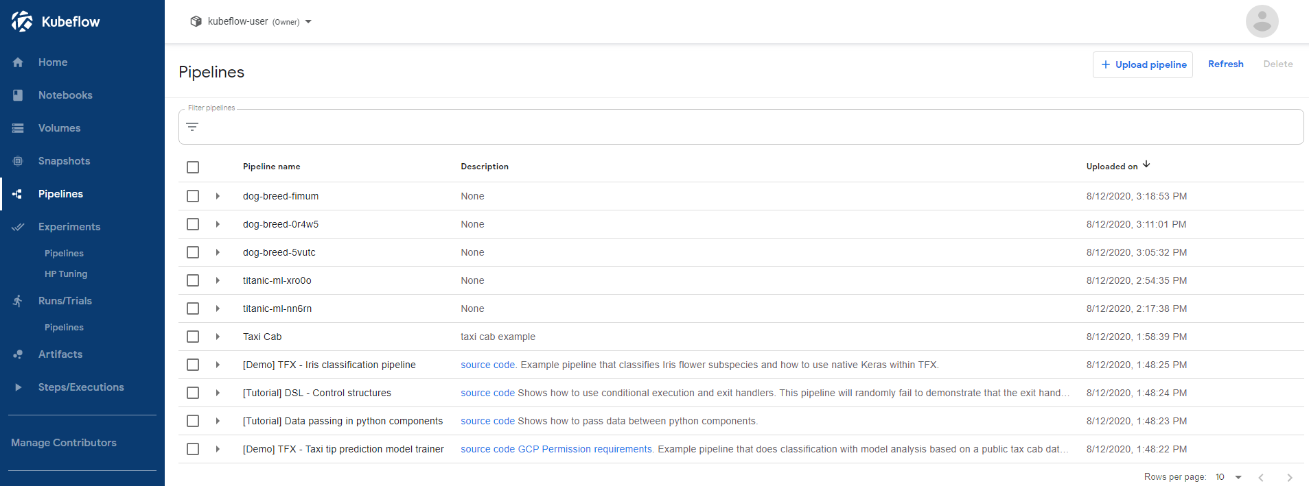
Once the file is downloaded to your laptop, go to Kubeflow Dashboard and open the Kubeflow Pipelines UI by clicking “Pipelines” on the left pane:
This will take you to the Kubeflow Pipelines UI:
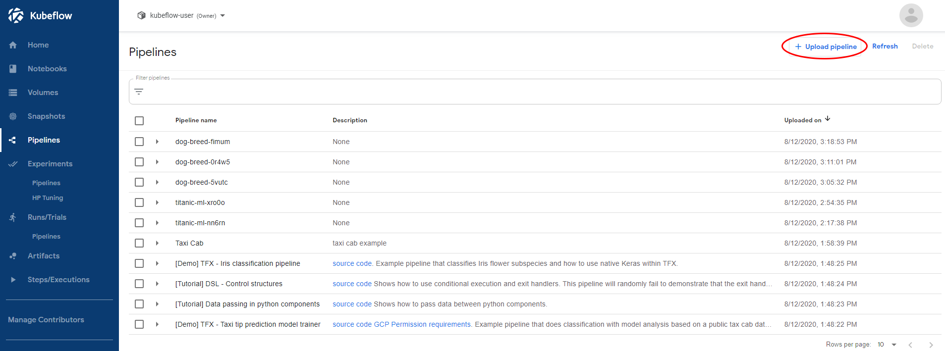
Click “+ Upload pipeline”:
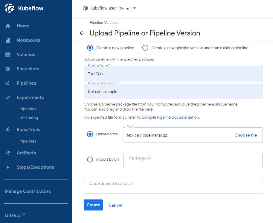
Choose a name and a description for your pipeline. Then click the “Upload a file” option and choose the .tar.gz file you downloaded locally. Finally, click “Create”.
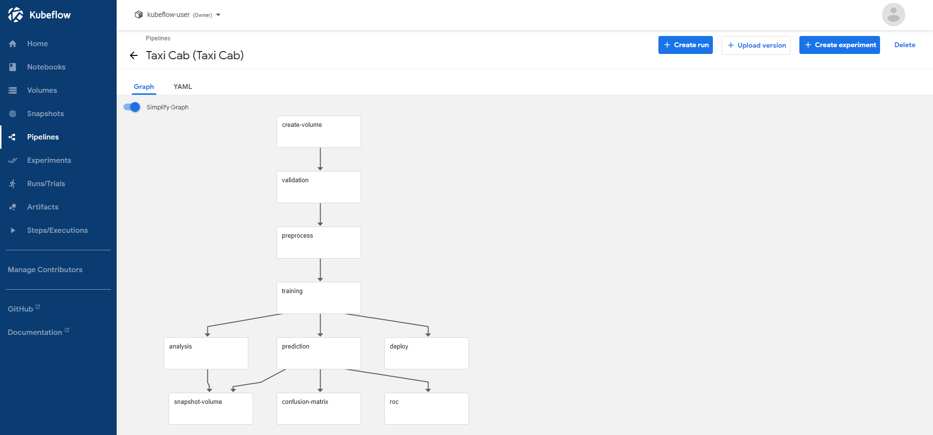
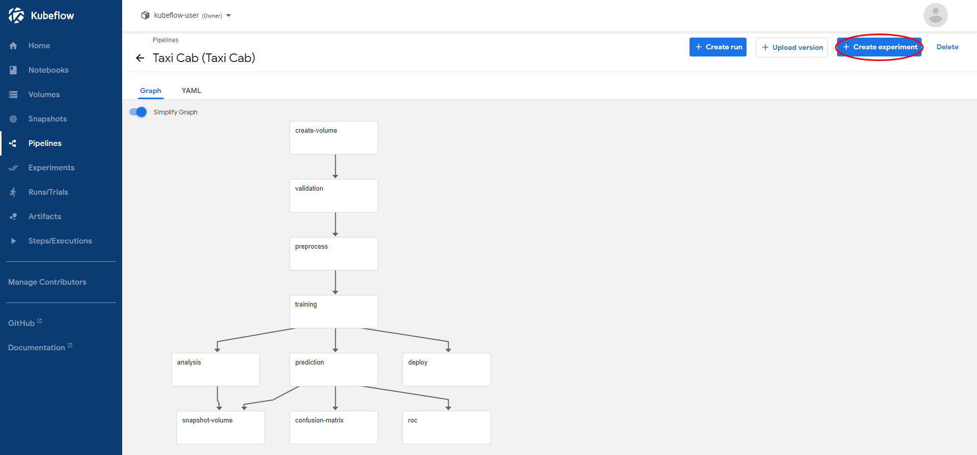
The pipeline should get uploaded successfully and you should be seeing its graph.
Create a new Experiment Run
Create a new Experiment by clicking “+ Create experiment”:
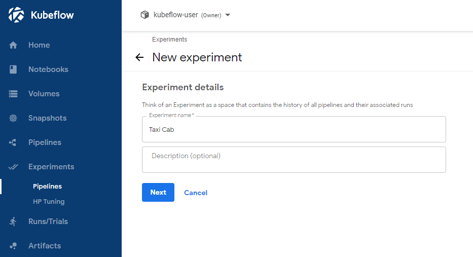
Choose an Experiment name, and click “Next”:
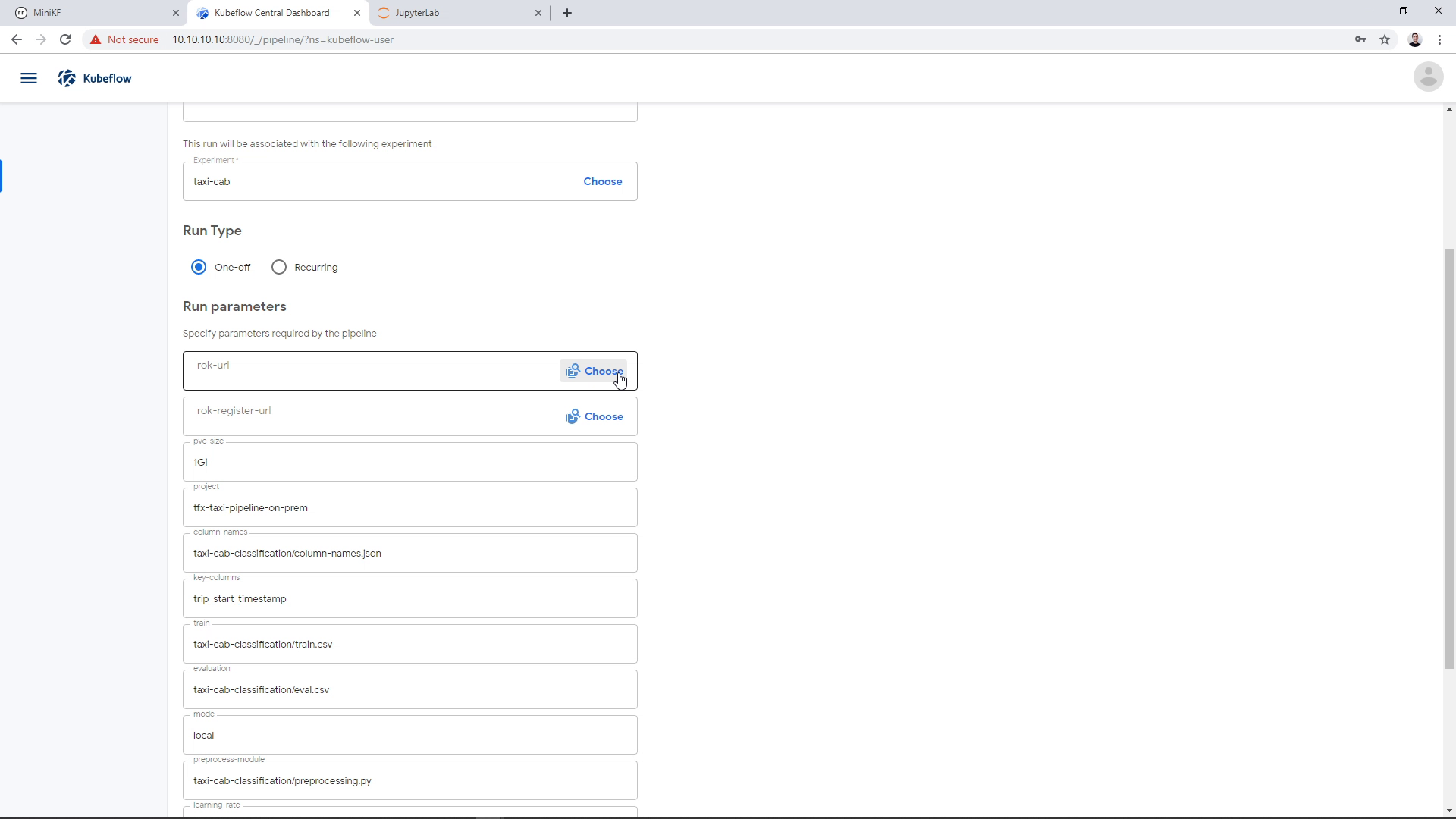
By clicking “Next”, the KFP UI sends you to the “Start a new run” page, where you are going to create a new Run for this Experiment. Enter a name for this Run (note that the Pipeline is already selected. If this is not the case, just select the uploaded Pipeline):

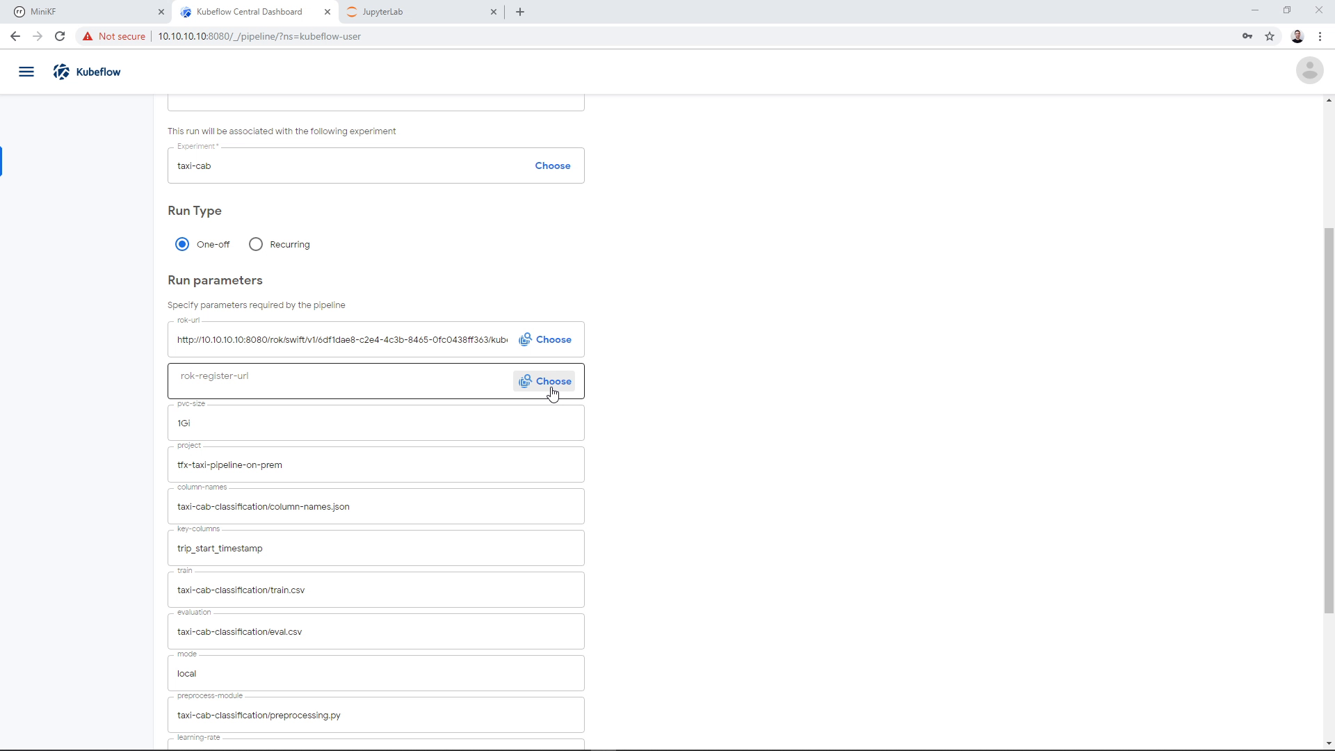
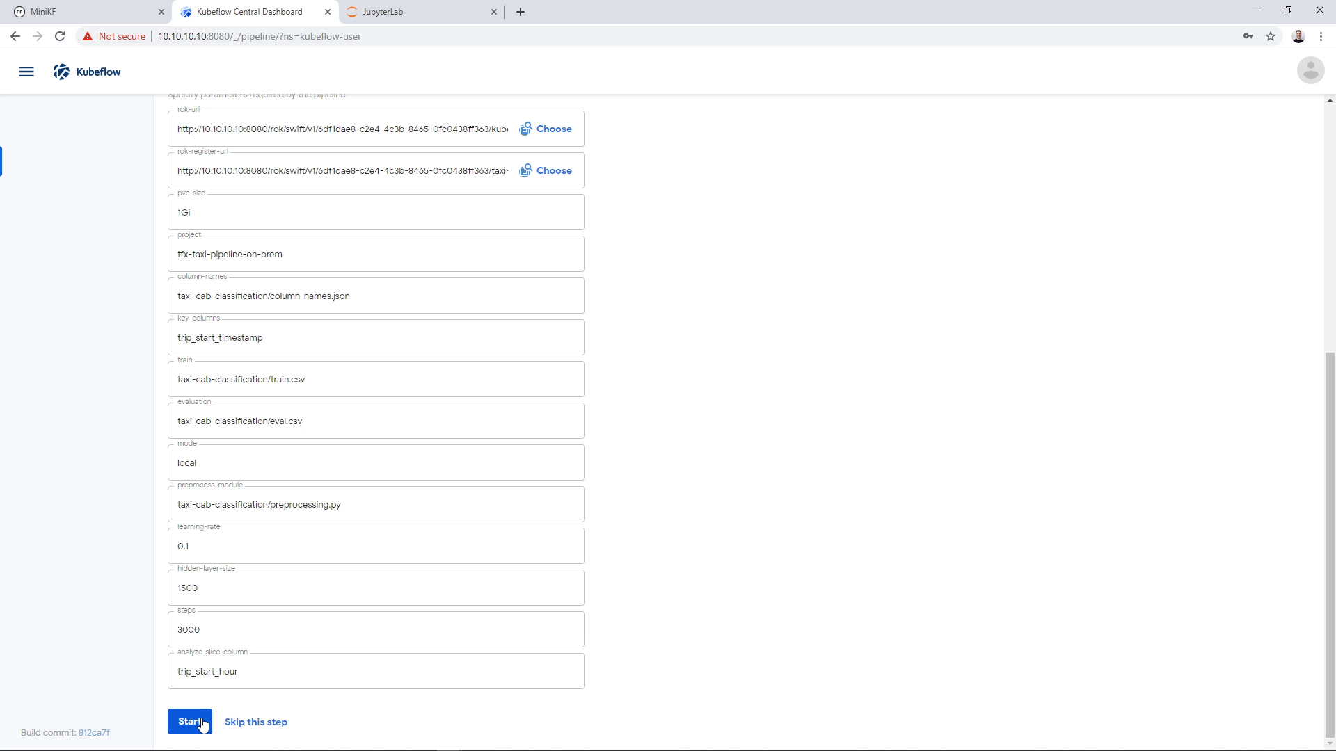
Note that the Pipeline’s parameters show up:

Seed the Pipeline with the Notebook’s Data Volume
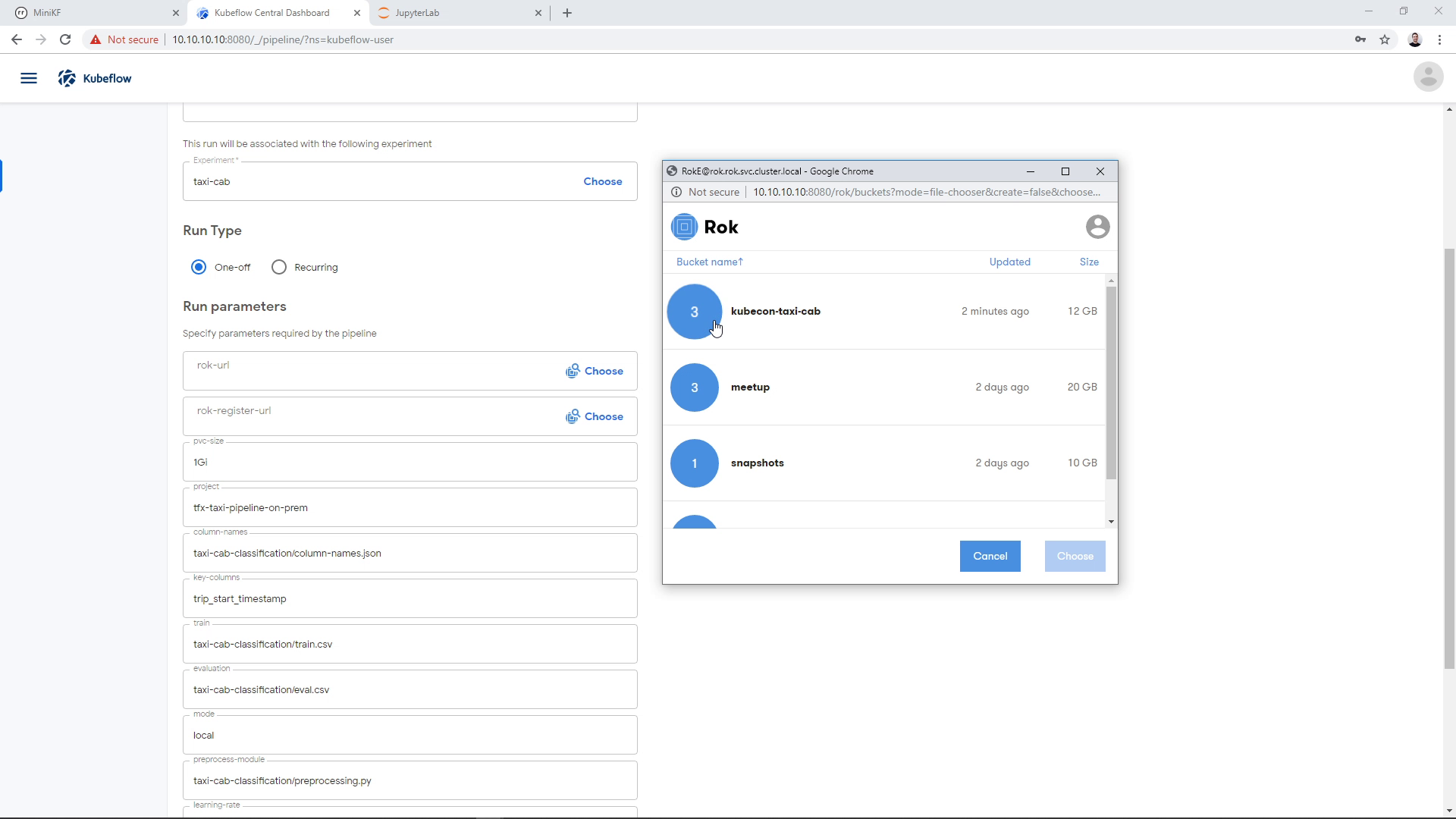
On the “rok-url” parameter we need to specify the snapshot of the Notebook Server’s Data Volume, which we created in the previous step. Click on “Choose” to open the Rok file chooser and select the snapshot of this Data Volume:
Enter inside the bucket you created previously:
Expand the file inside the bucket:
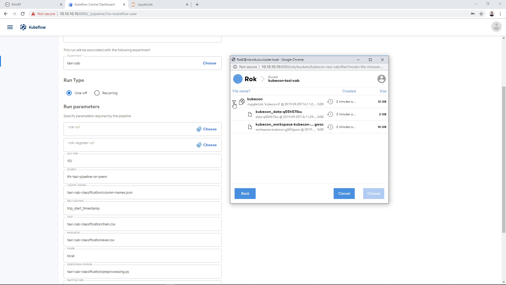
Find the snapshot of the Data Volume and click on it. Make sure that you have chosen the Data Volume and not the Workspace Volume:
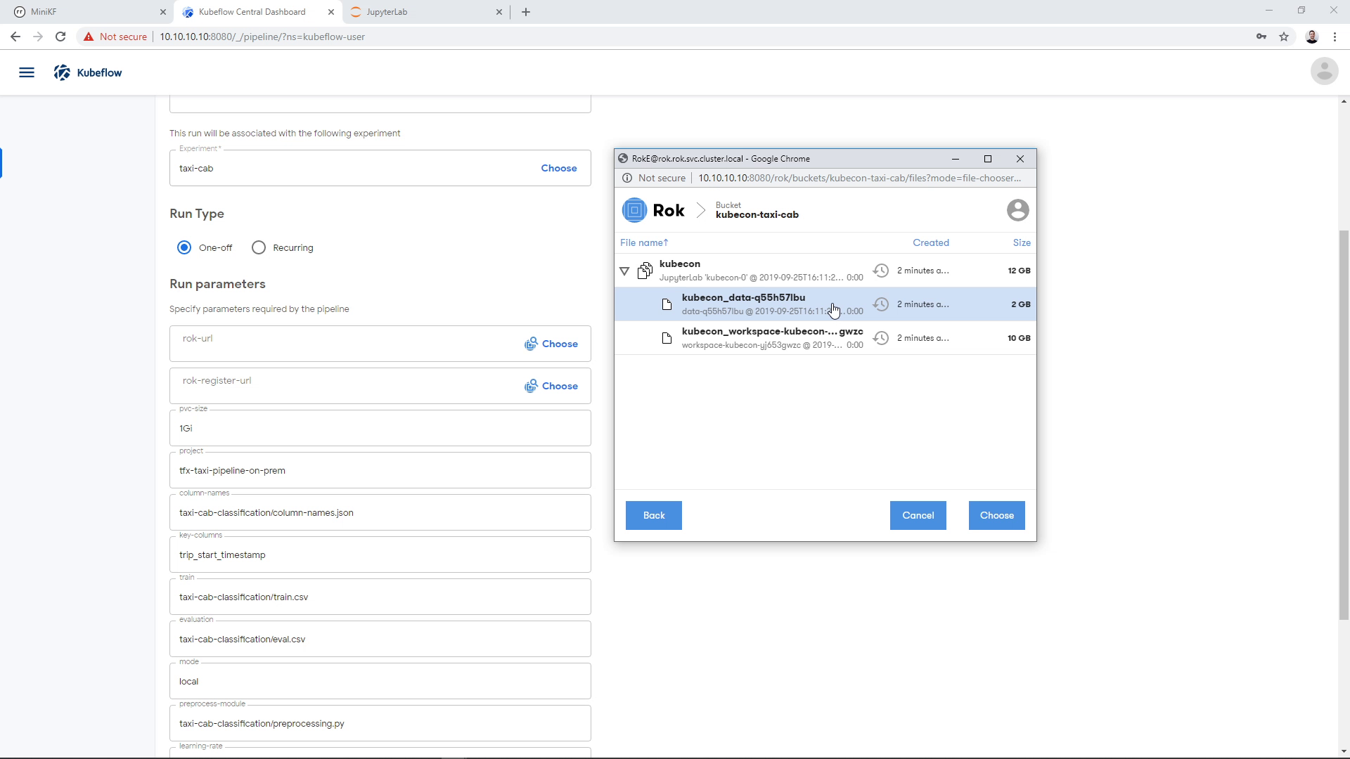
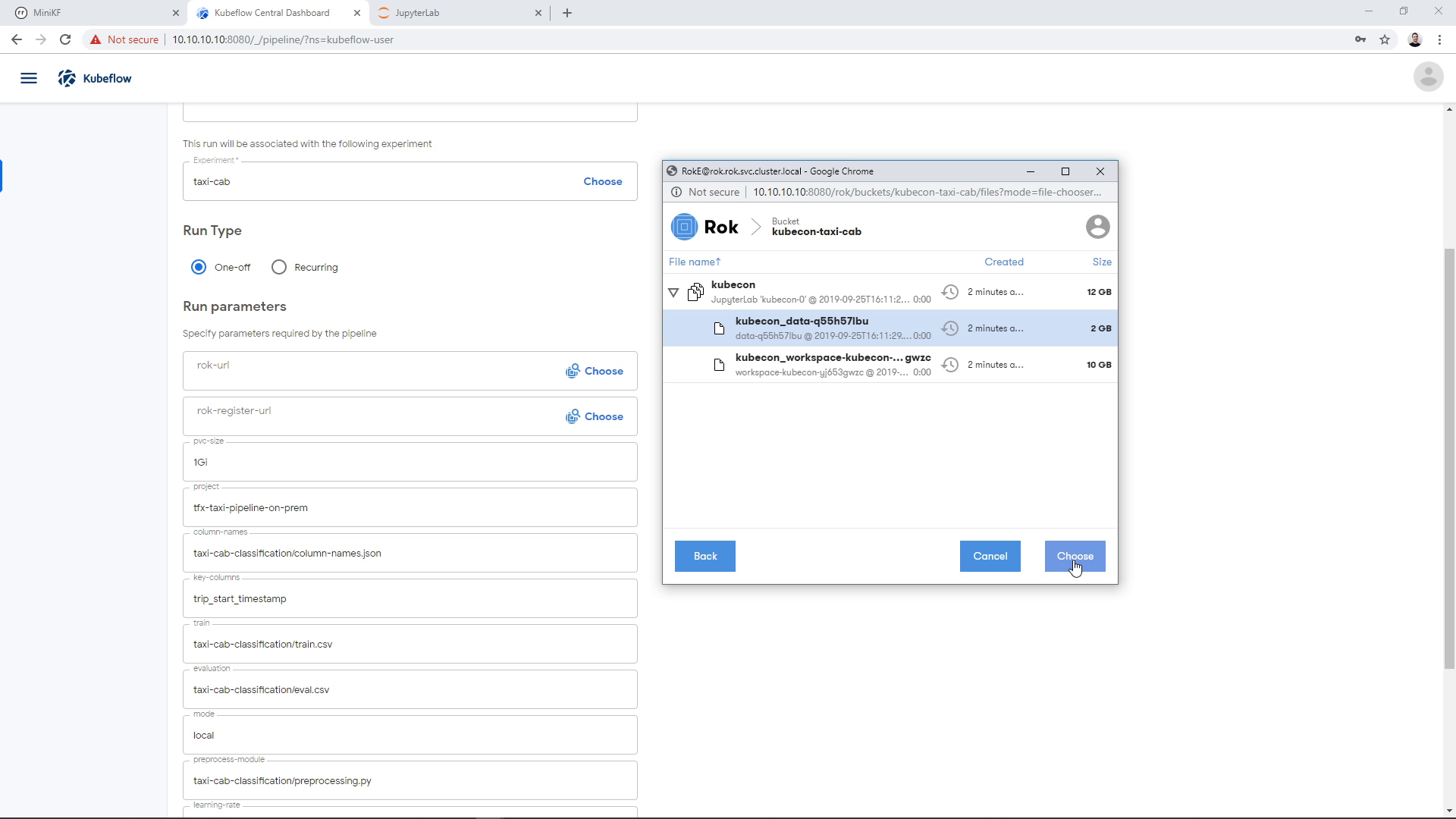
Then click on “Choose”:
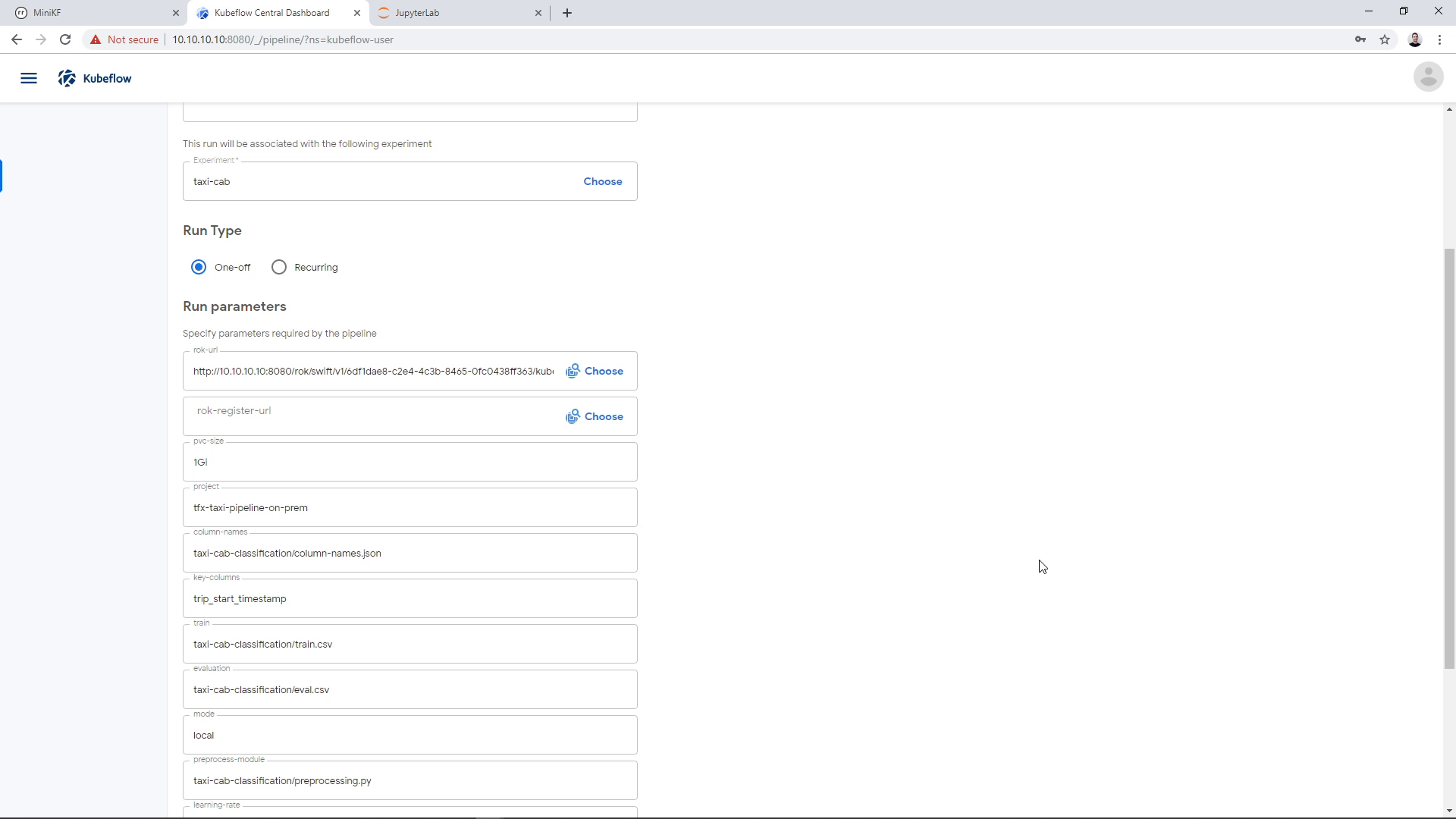
The Rok URL that corresponds to the Data Volume snapshot appears on the corresponding parameter field:
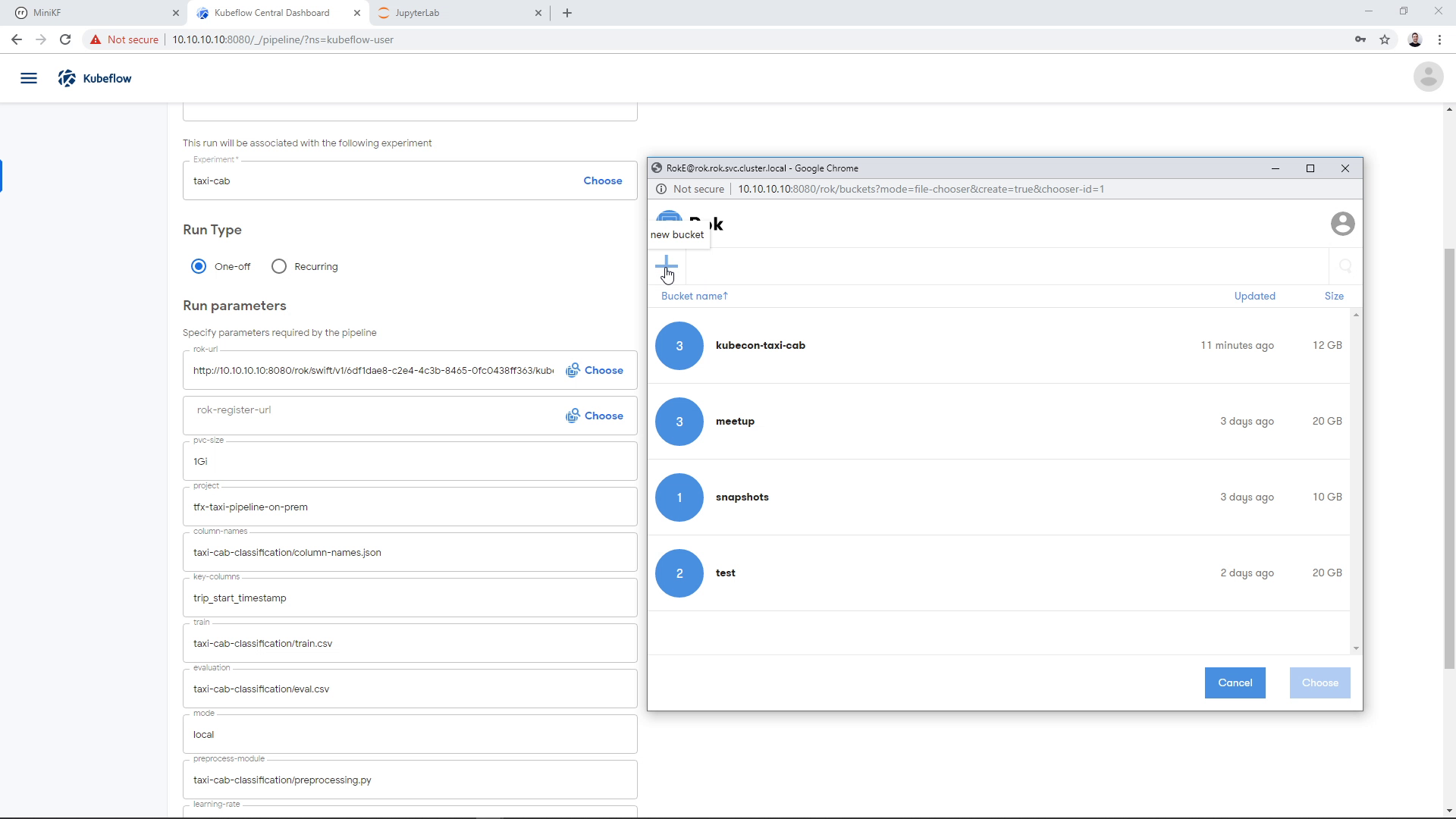
Select a bucket to store the pipeline snapshot
On the “rok-register-url” parameter we need to choose where we are going to store the pipeline snapshot. For that, we need to specify a bucket and a name for the file (snapshot) that is going to be created. We can select an existing bucket and an existing file. This would create a new version of this file. Here, we will create a new bucket and a new file. First, we click on the “Choose” button to open the Rok file chooser:
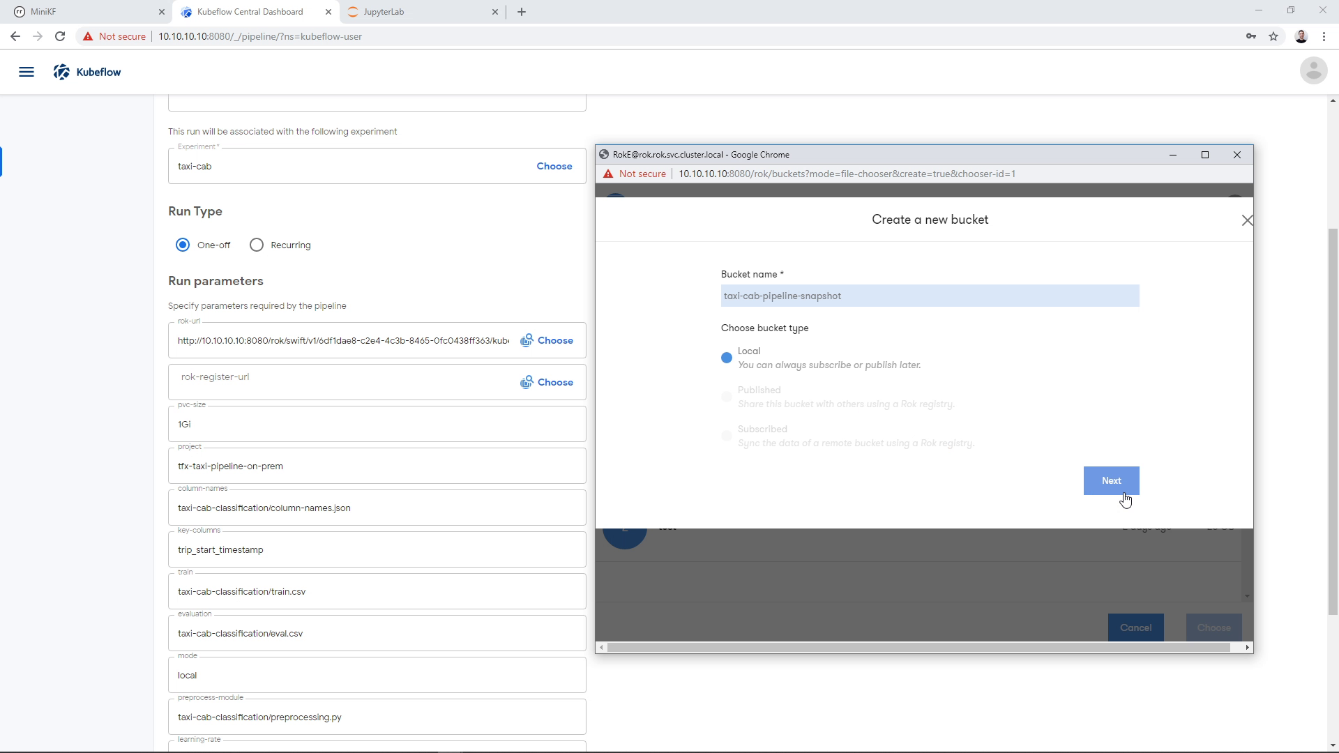
We create a new bucket:
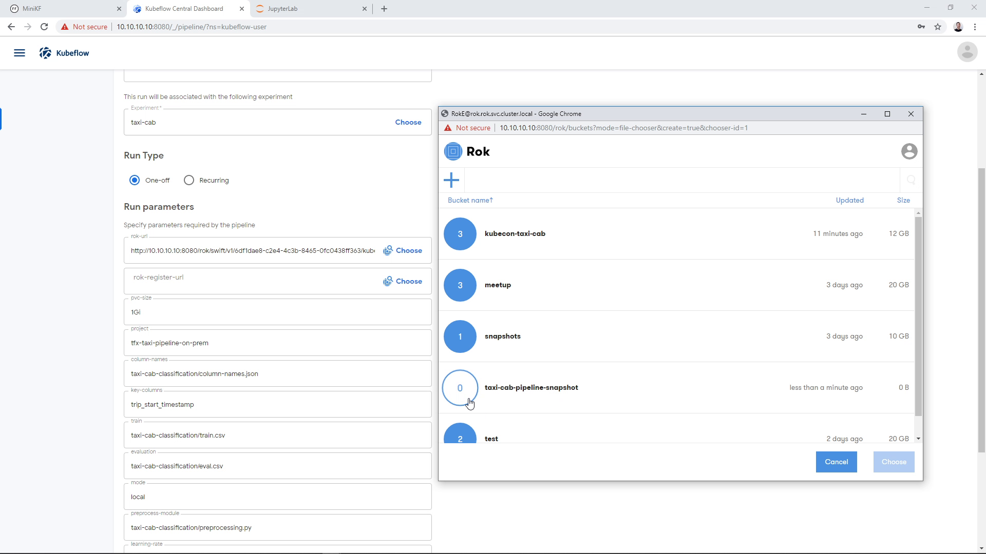
We give it a name and click “Next”:
Then we enter the bucket:
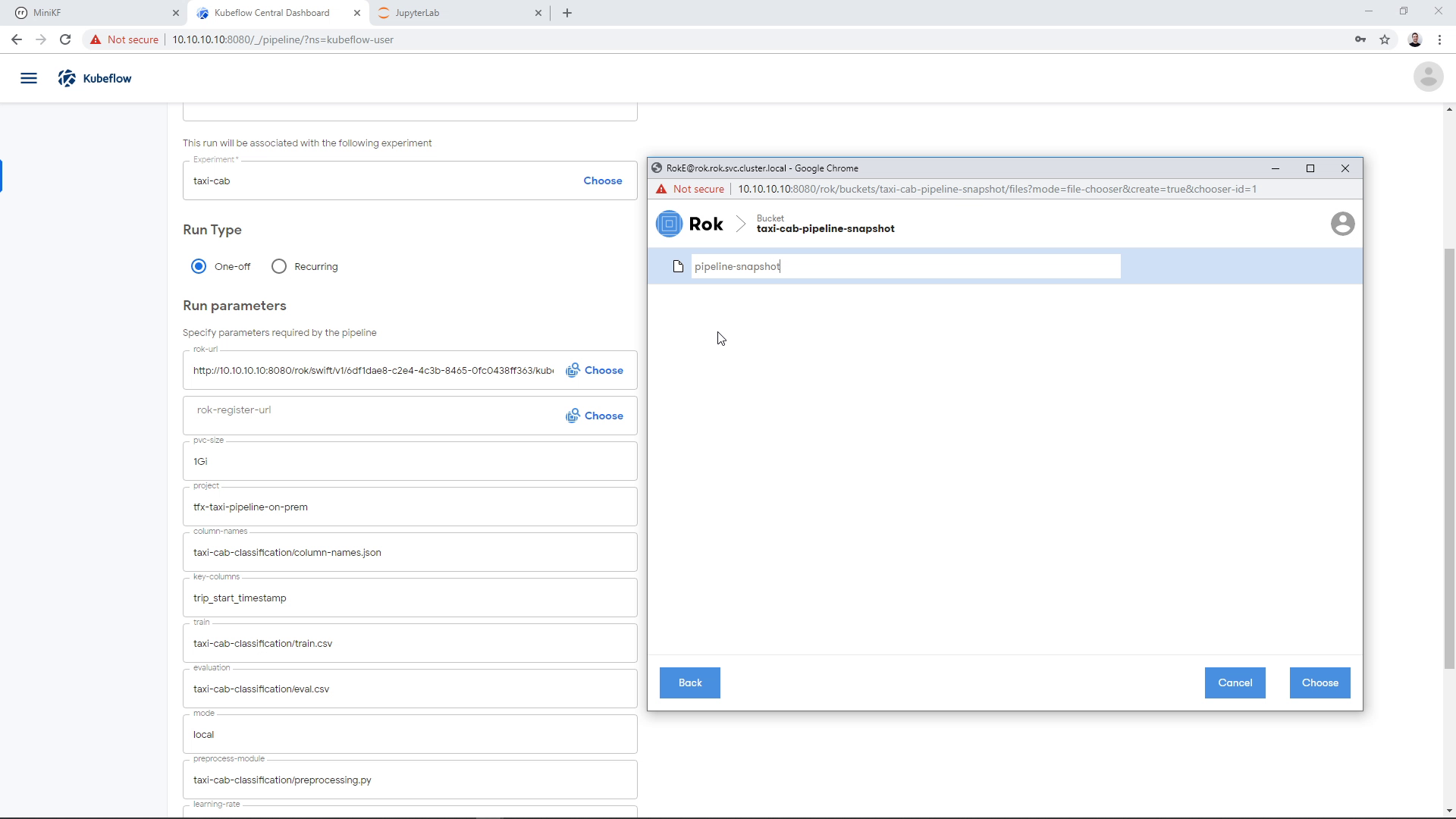
We create a new file:
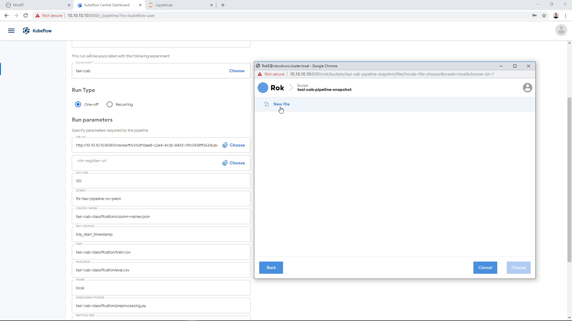
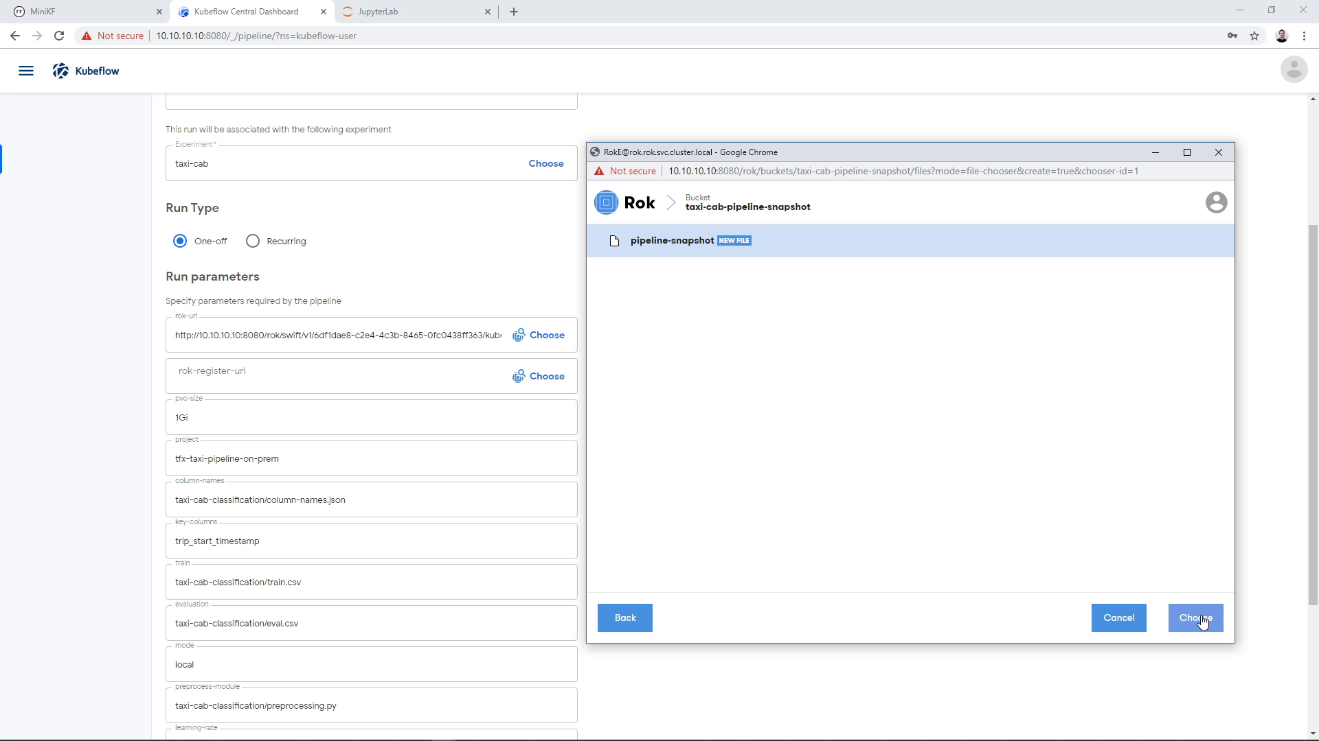
We give it a name:
And click “Choose”:
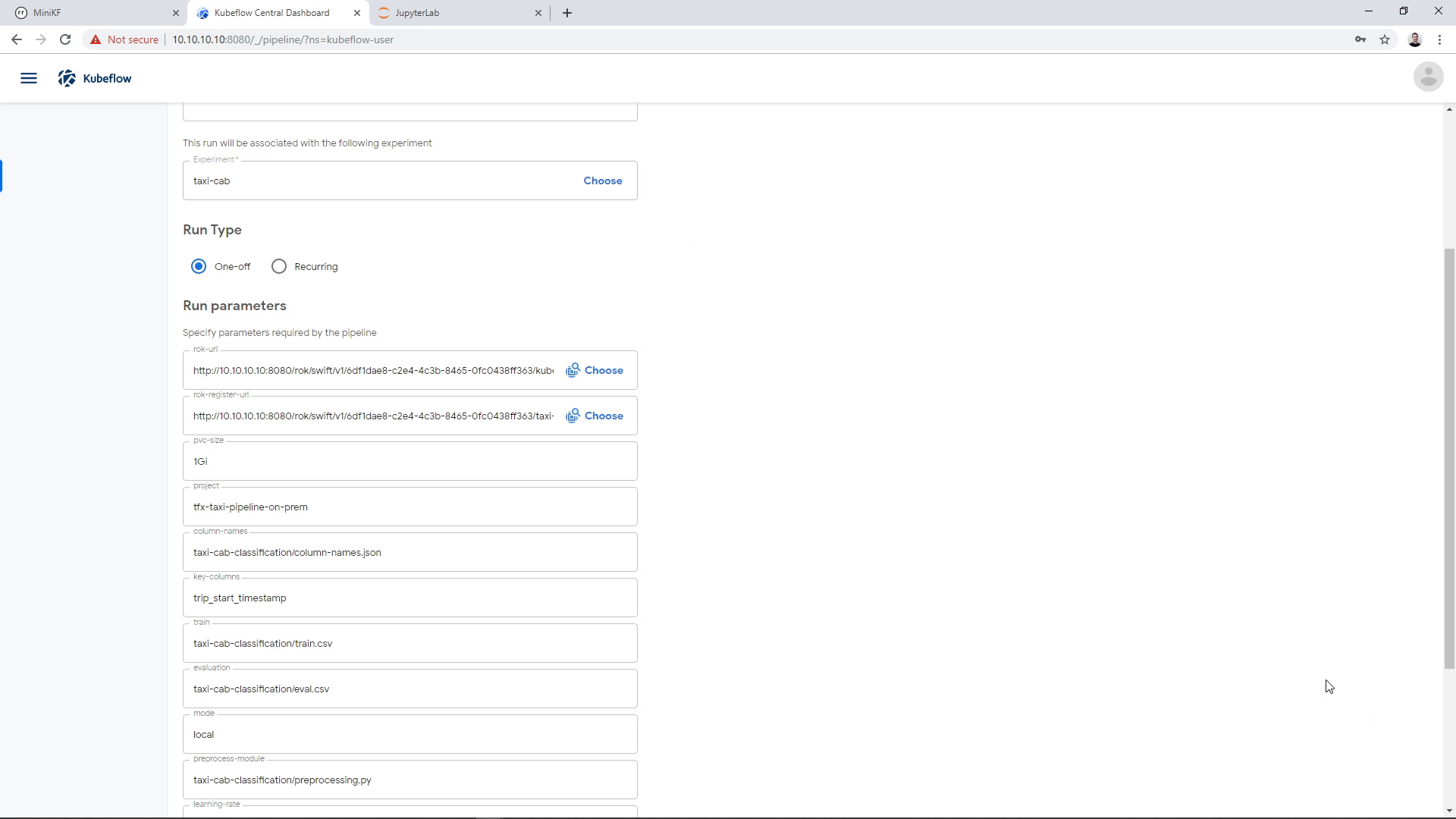
The Rok URL that corresponds to the pipeline snapshot appears on the corresponding parameter field:
Run the Pipeline
Now that we have defined the data to seed the pipeline and the file to store the pipeline snapshot, we can run the pipeline. We are leaving all other parameters as is, and click “Start”:
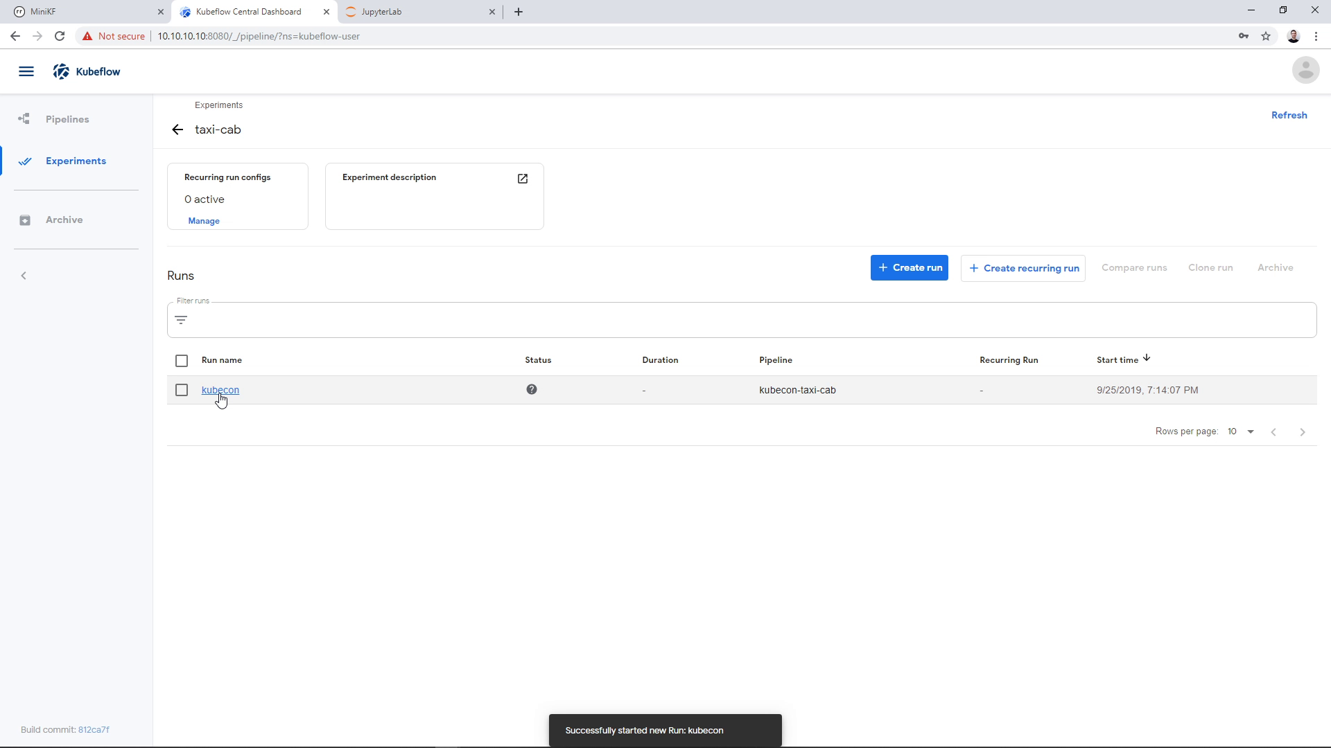
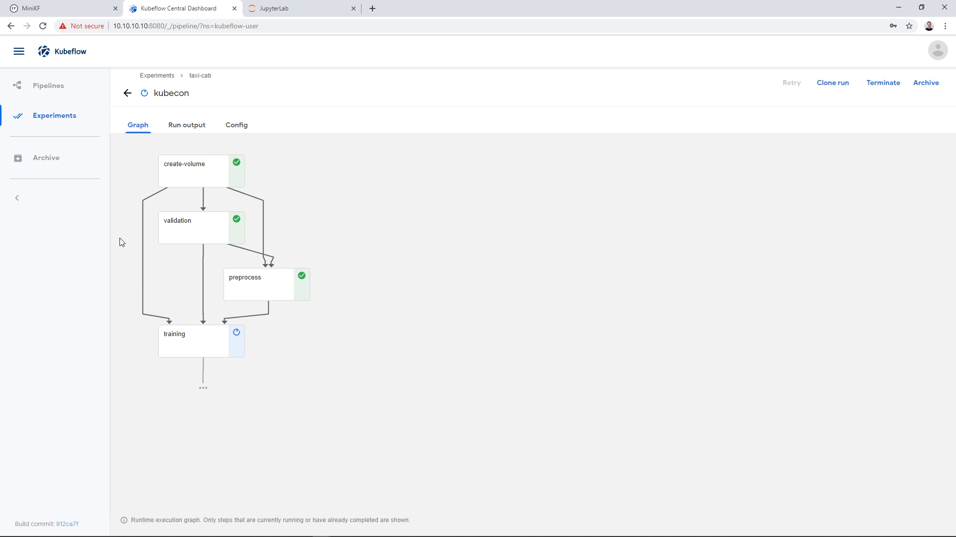
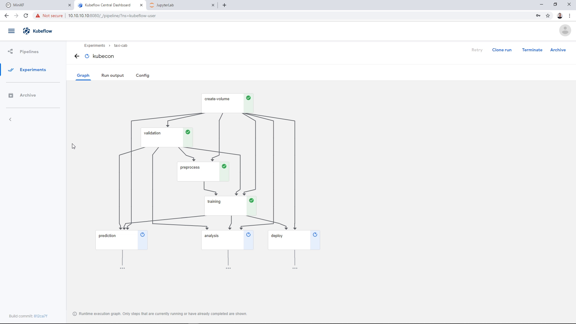
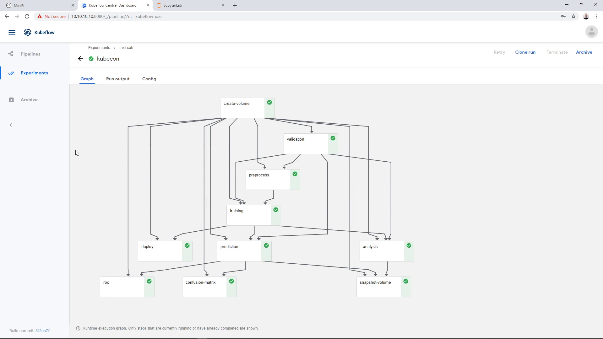
Now, click on the Run you created to view the progress of the Pipeline:
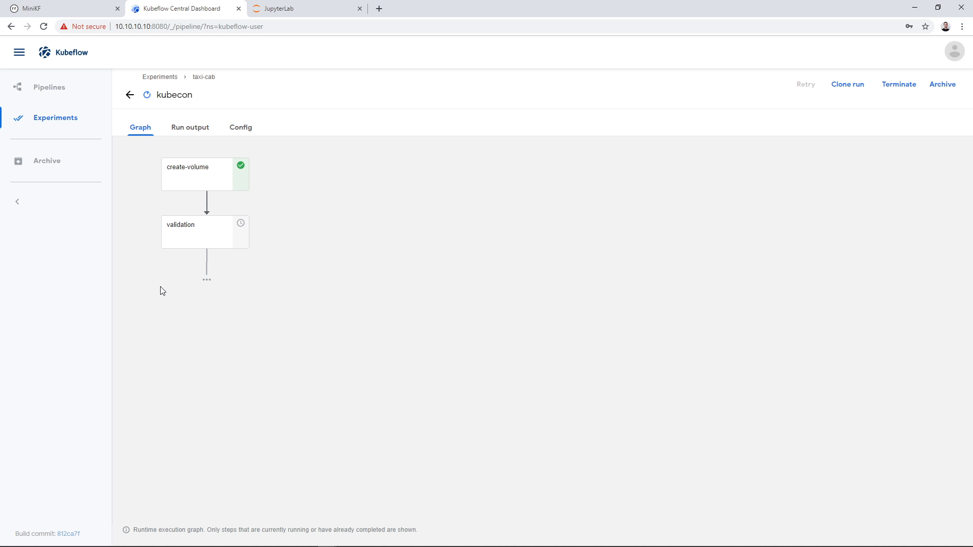
As the Pipeline runs, we see the various steps running and completing successfully. The Pipeline is going to take 10 to 30 minutes to complete, depending on your laptop specs. During the first step, Rok will instantly clone the snapshot we provided, for the next steps to use it:
Note: If the validation step fails with:
/mnt/taxi-cab-classification/column-names.json;
No such file or directory
then you have to make sure that you have given the name “data” to your Data Volume. If not, then make sure that you amended the command of cell 3 accordingly, so that the data of the pipeline gets stored to your Data Volume.
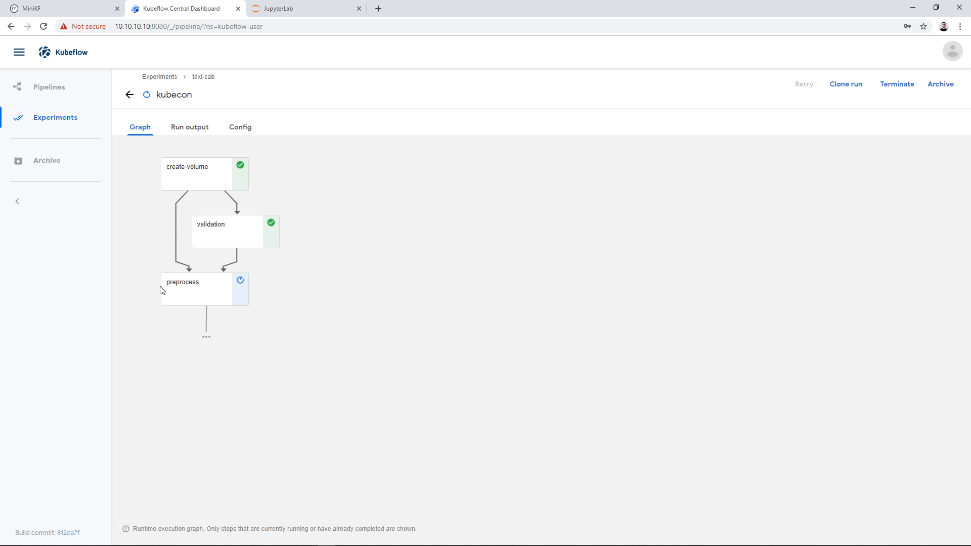
The training step is going to take a few minutes:
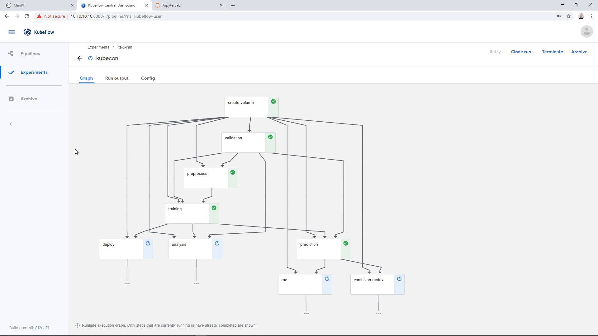
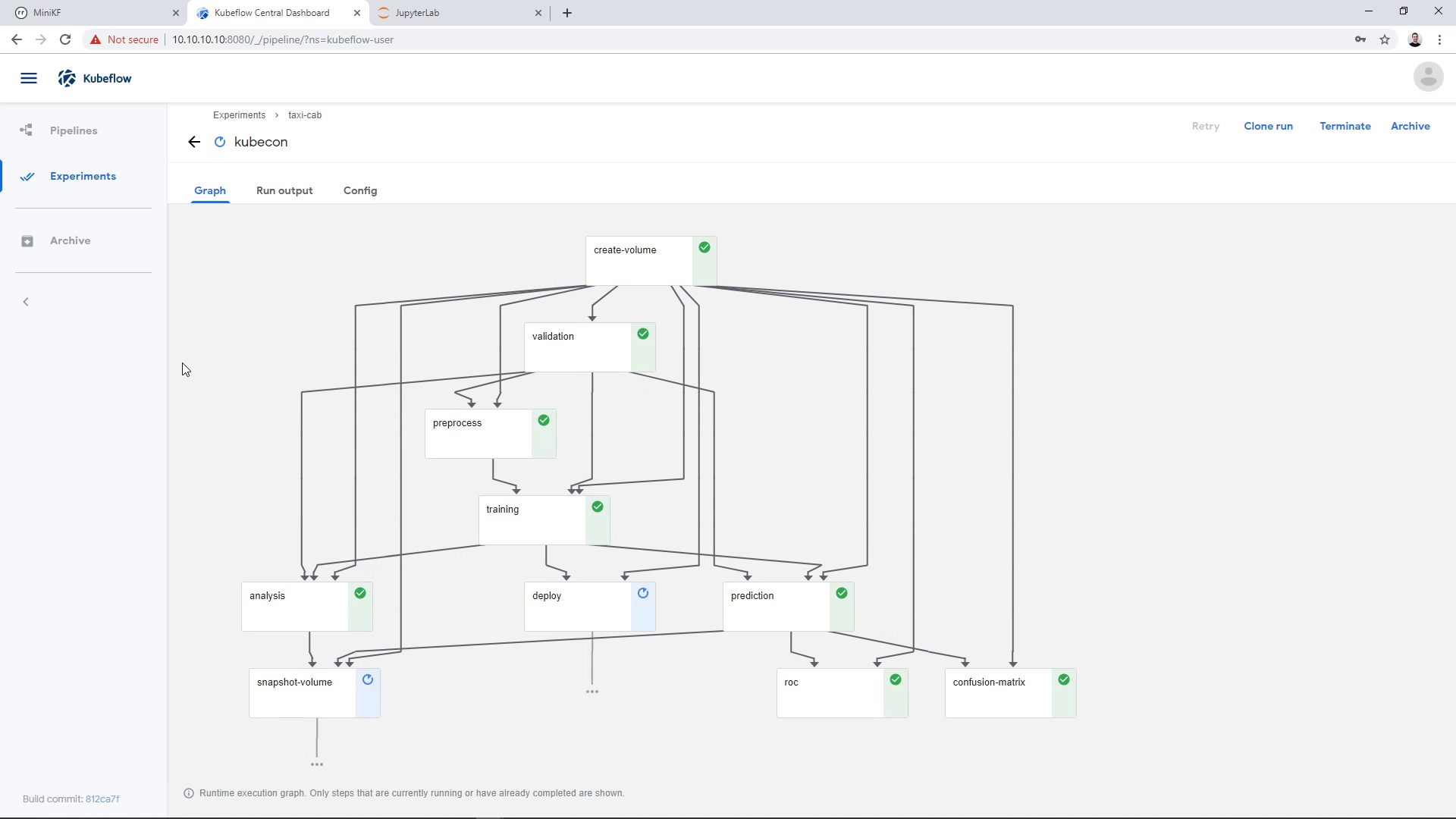
Pipeline snapshot with Rok
As a last step, Rok will automatically take a snapshot of the pipeline, so that we can later attach it to a Notebook and do further exploration of the pipeline results. You can see this step here:
Update: in later versions of MiniKF, the `deploy` step will fail. This happens, because this step assumes the pipeline runs inside the `kubeflow` namespace.
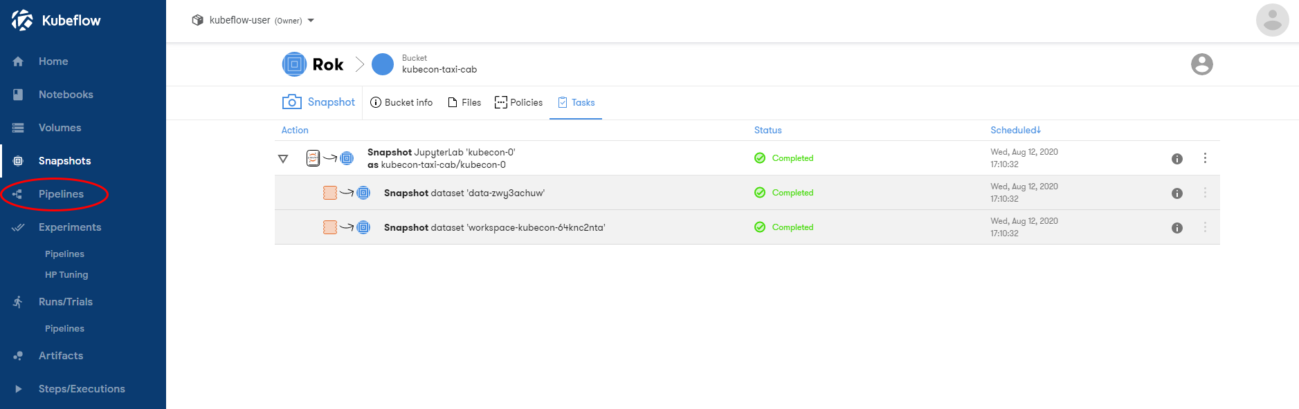
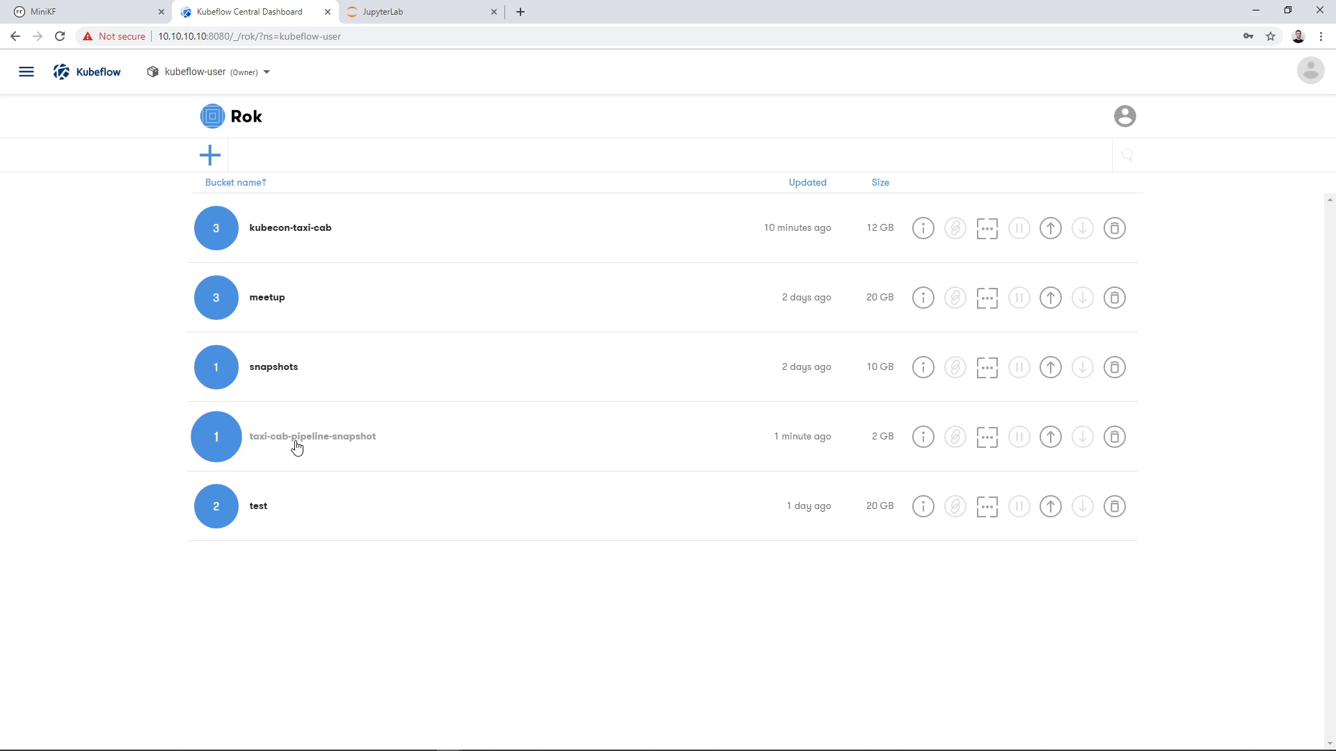
If we go back to the Rok UI, we can see the snapshot that was taken during the pipeline run. We go to the Rok UI landing page:
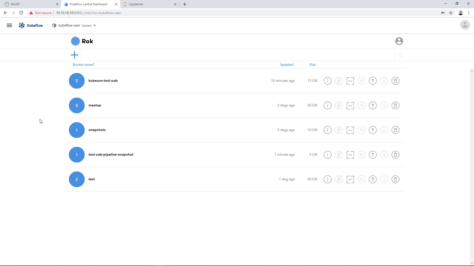
We find the bucket that we chose earlier to store the snapshot, in this case “taxi-cab-pipeline-snapshot”:
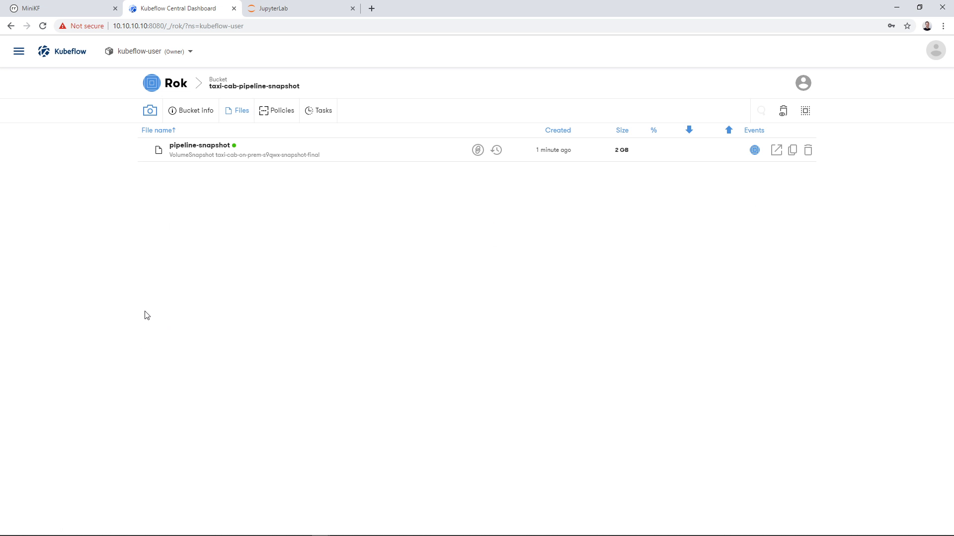
And we see the pipeline snapshot that has the name that we chose earlier, in this case “pipeline-snapshot”:
Explore pipeline results inside a Notebook
To explore the pipeline results, we can create a new Notebook and attach it the pipeline snapshot. The Notebook will use a clone of this immutable snapshot. This means that you can do further exploration and experimentation using this Data Volume, without losing the results that the pipeline run produced.
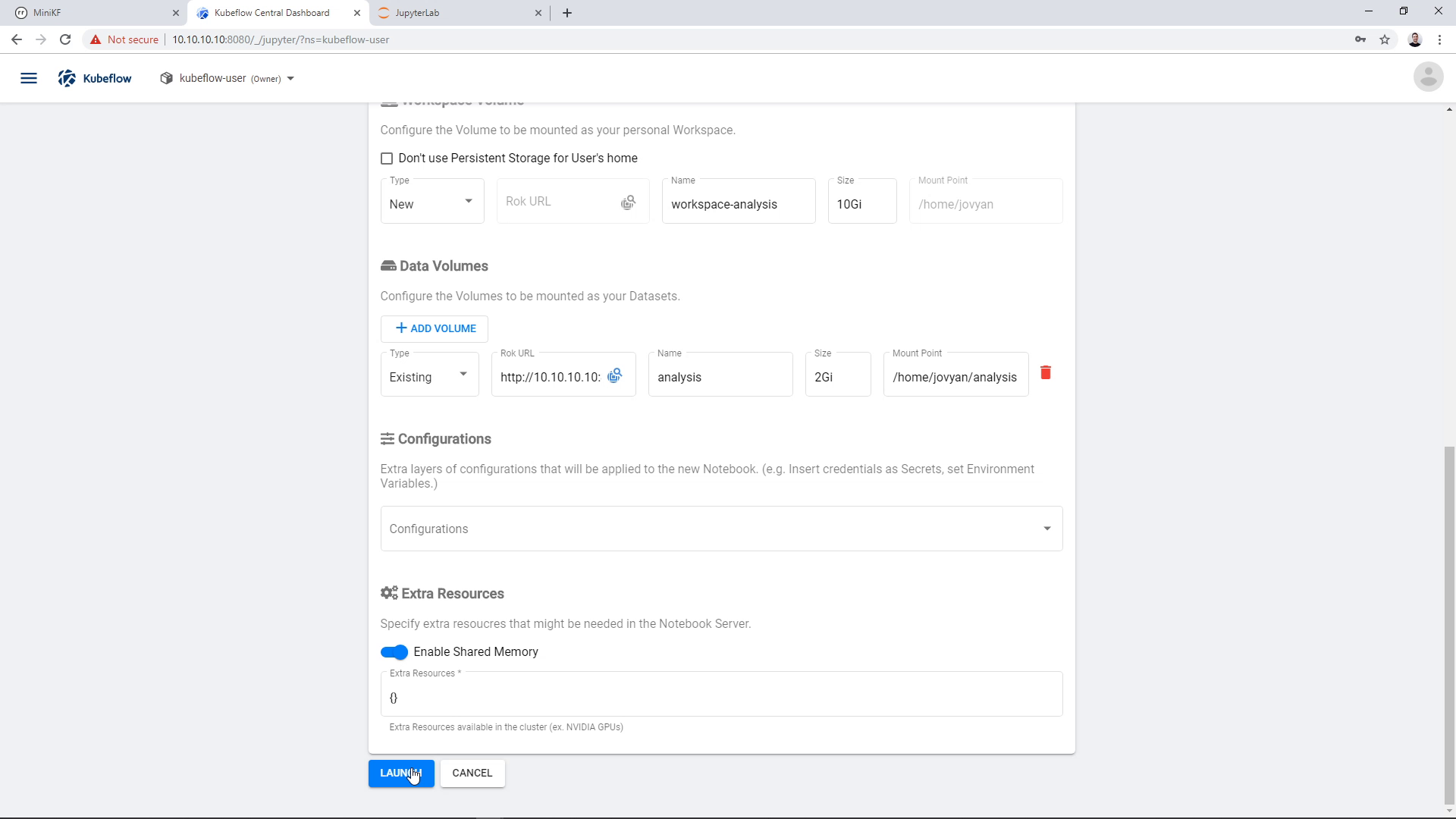
To do this, we create a new Notebook Server and add an existing Data Volume. Here, the volume will be the pipeline snapshot that lives inside Rok. We go to the Notebook Manager UI and click “New Server”:
Then, we enter a name for the new Notebook Server, and select Image, CPU, and RAM:
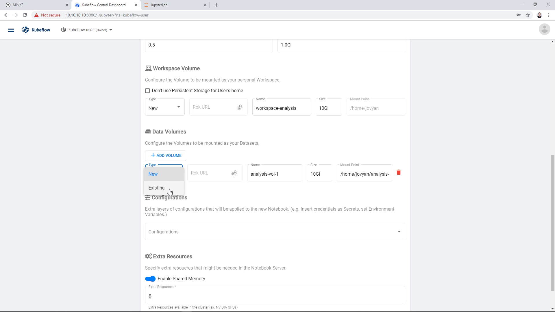
To add an existing Data Volume, click on “Add Volume”:
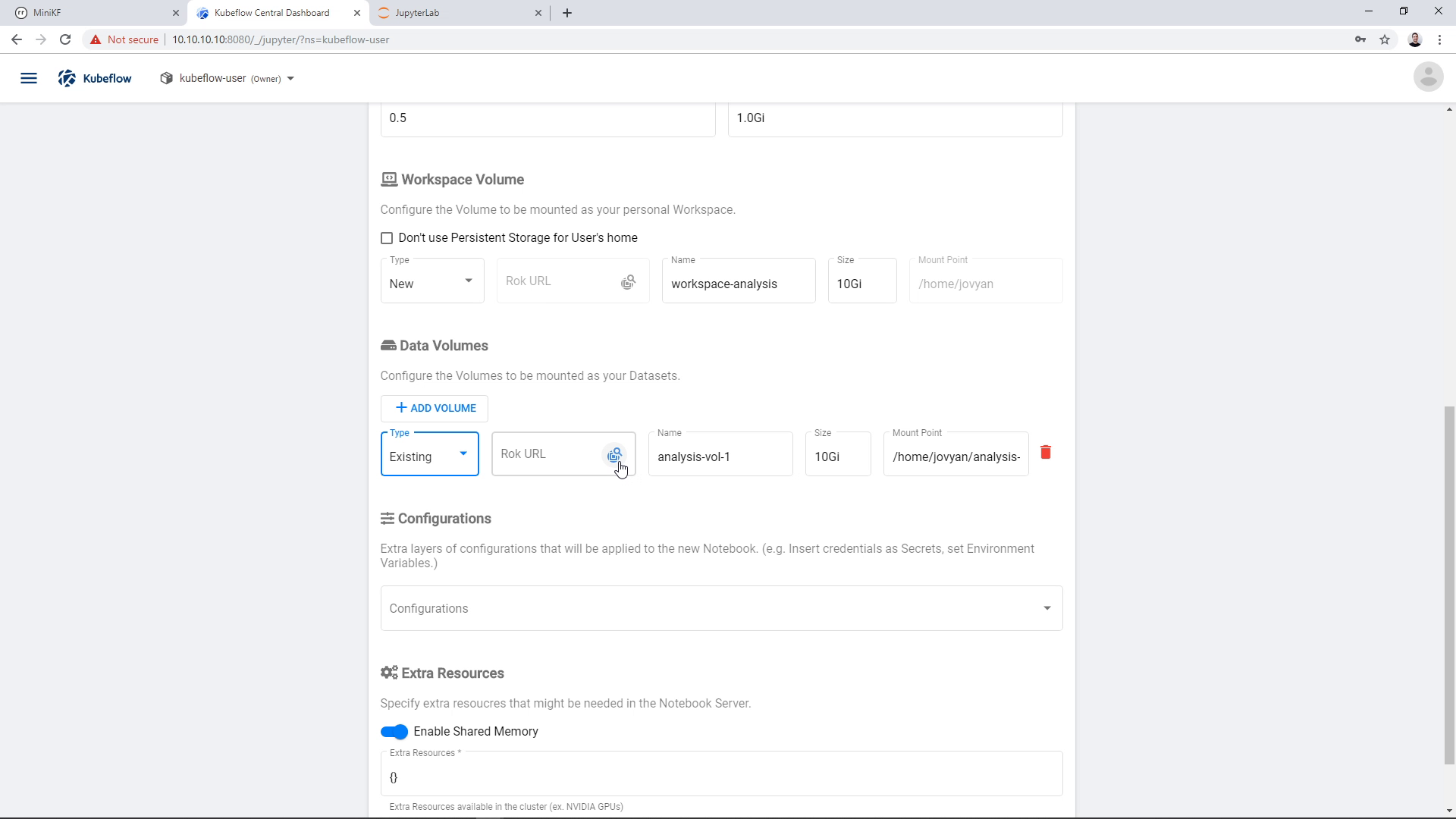
Then change its type to “Existing”:
Now, we will use the Rok file chooser to select the snapshot that was taken during the pipeline run. This snapshot contains the pipeline results. The Notebook will use a clone of this immutable snapshot, so you can mess with the volume without losing any of your critical data.
We click on the Rok file chooser icon and open the file chooser:
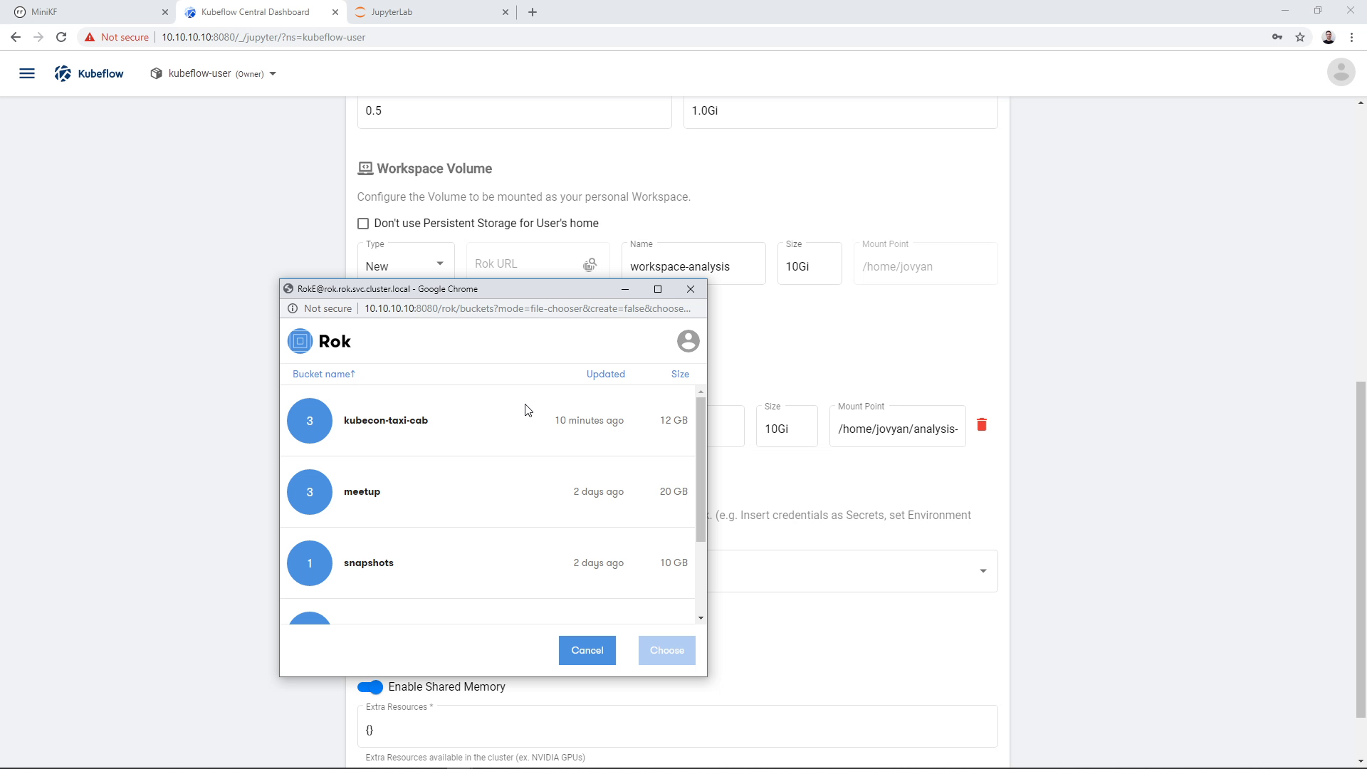
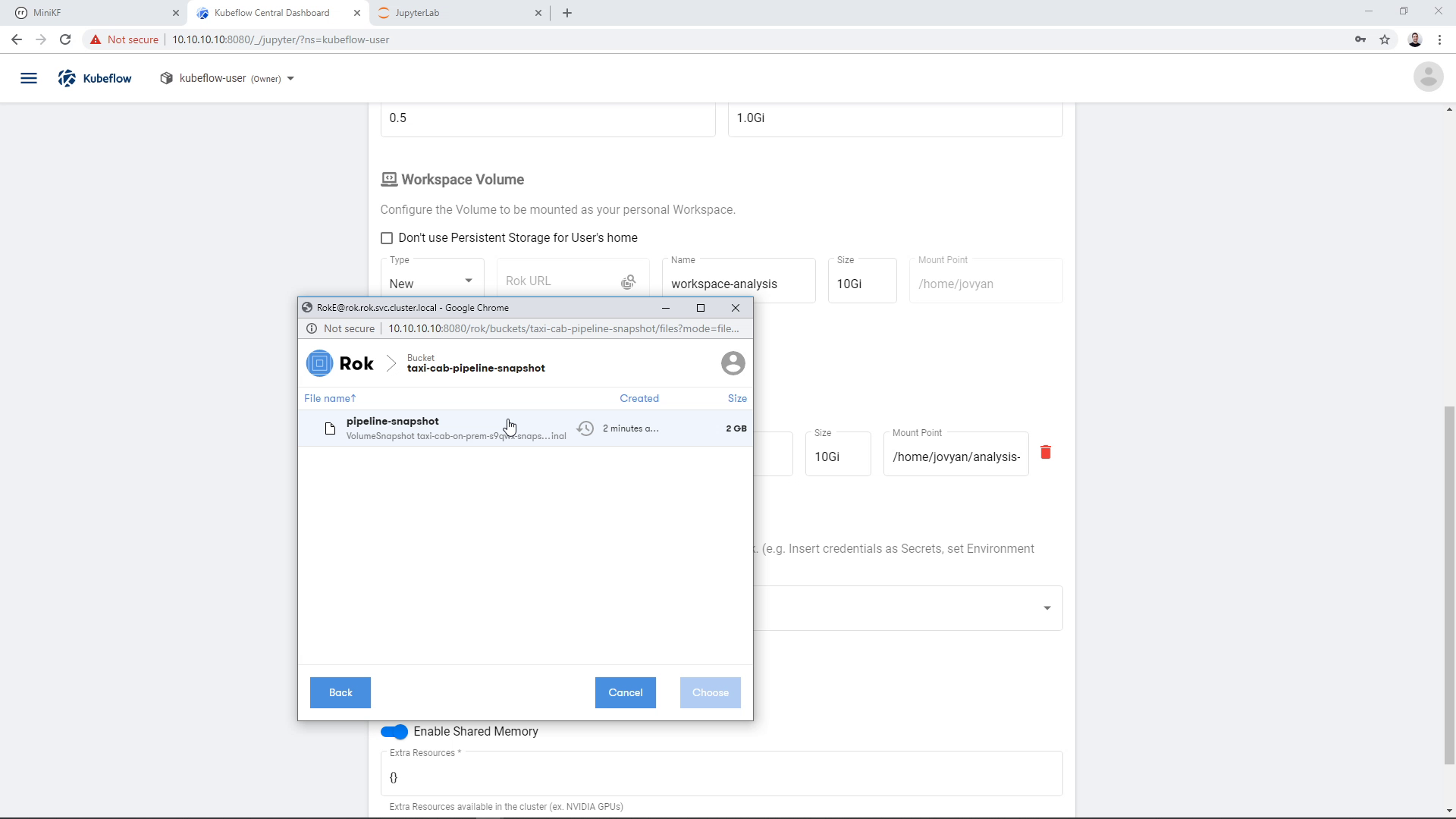
We find the bucket that we chose earlier to store the snapshot, in this case “taxi-cab-pipeline-snapshot”:
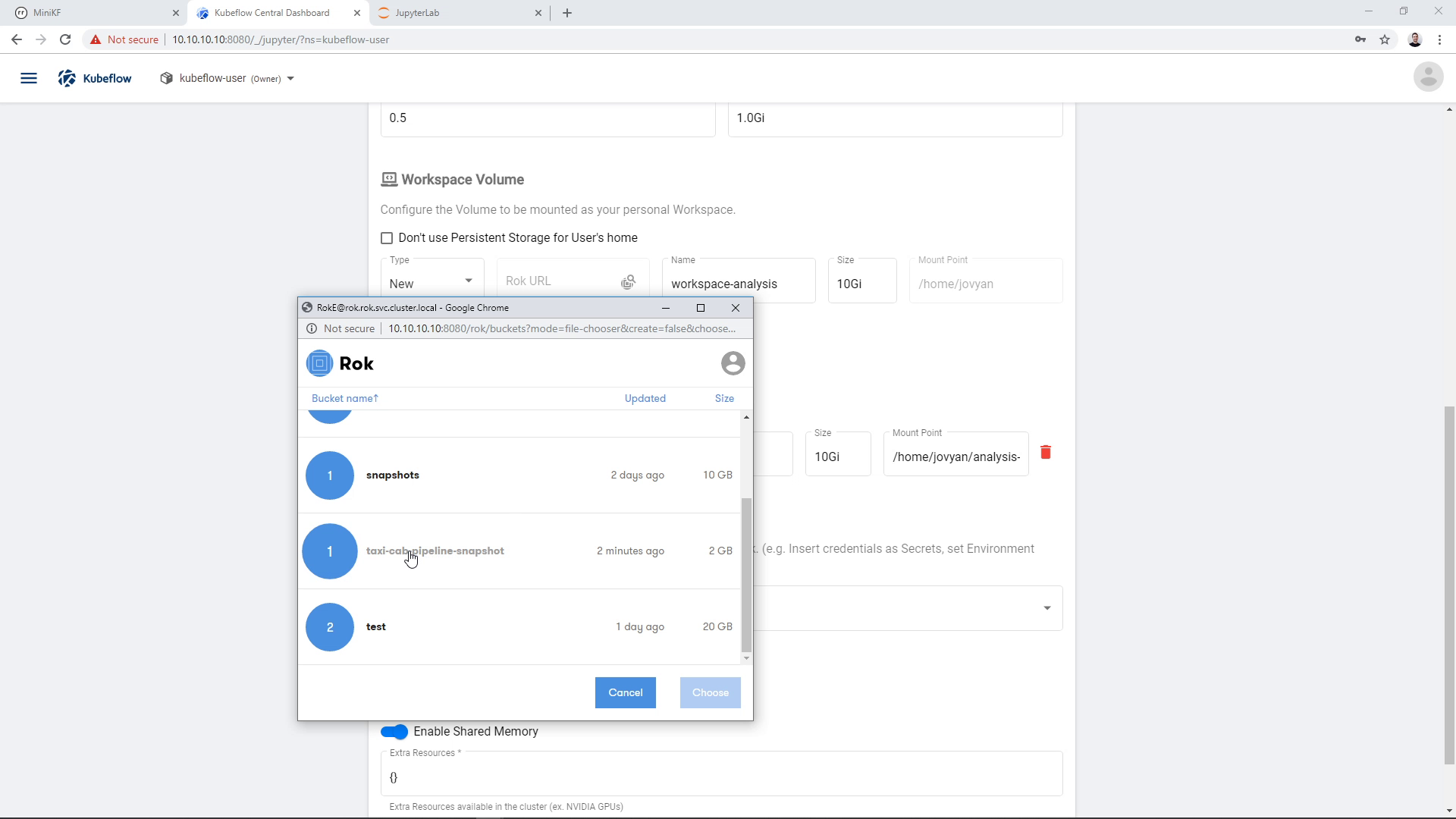
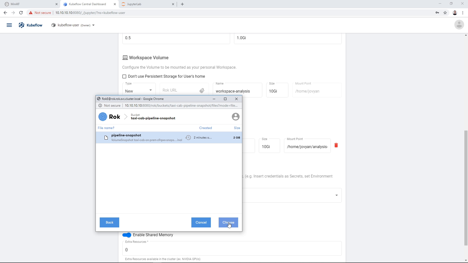
We click on the file (snapshot) that we created during the pipeline run, in this case “pipeline-snapshot”:
And then click “Choose”:
The Rok URL that corresponds to this snapshot appears in the “Rok URL” field:
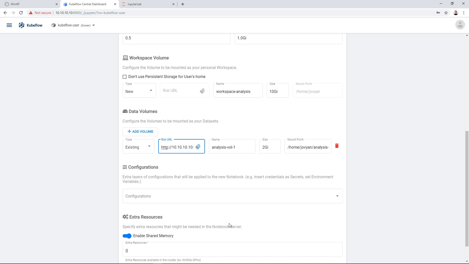
You can change the name of the volume if you wish. Here, we change it to “analysis”:
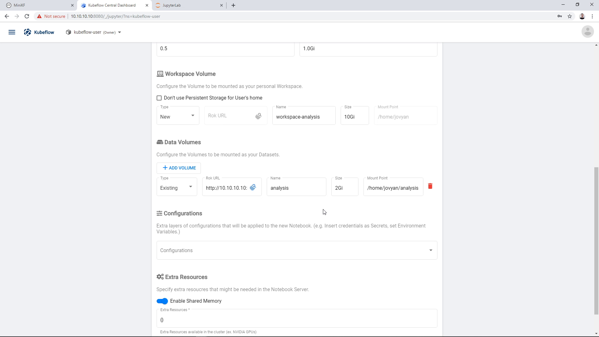
Then, we click “Launch”:
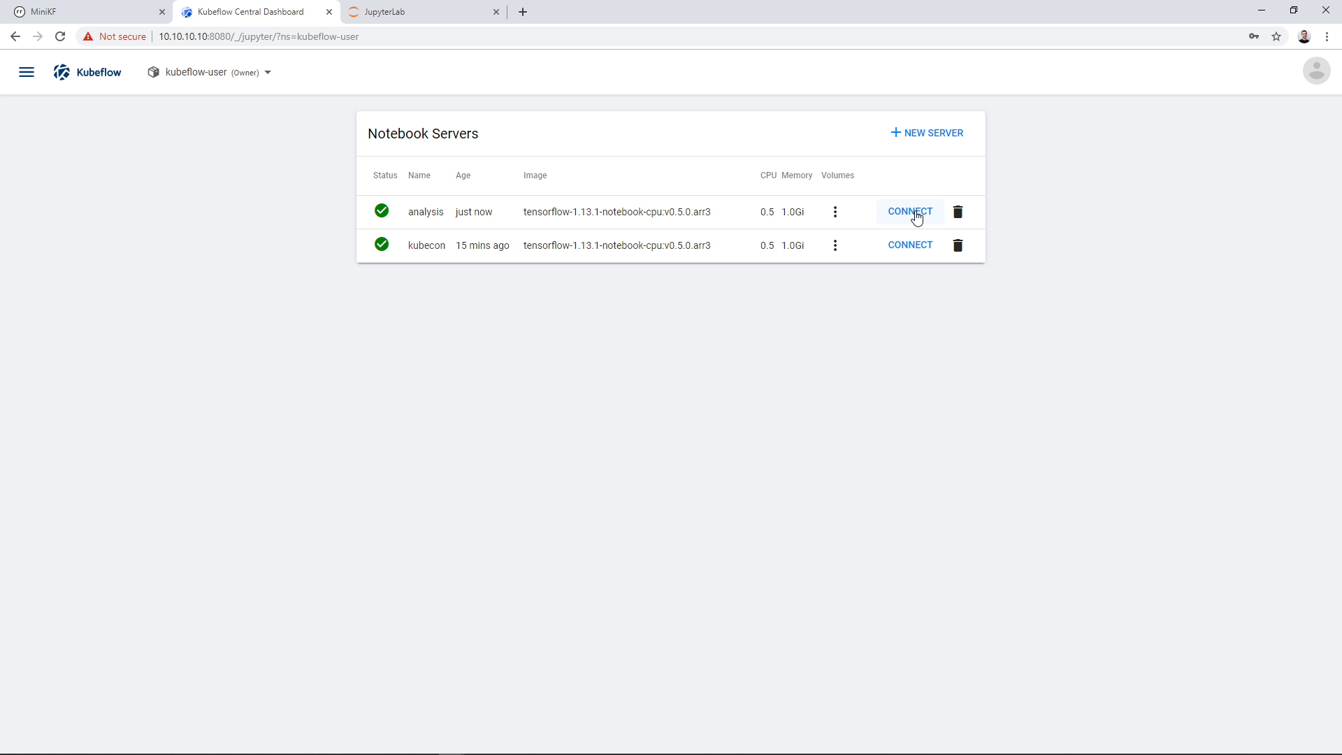
A new Notebook Server appears in the Notebook Manager UI. Click on “Connect” to go this JupyterLab:
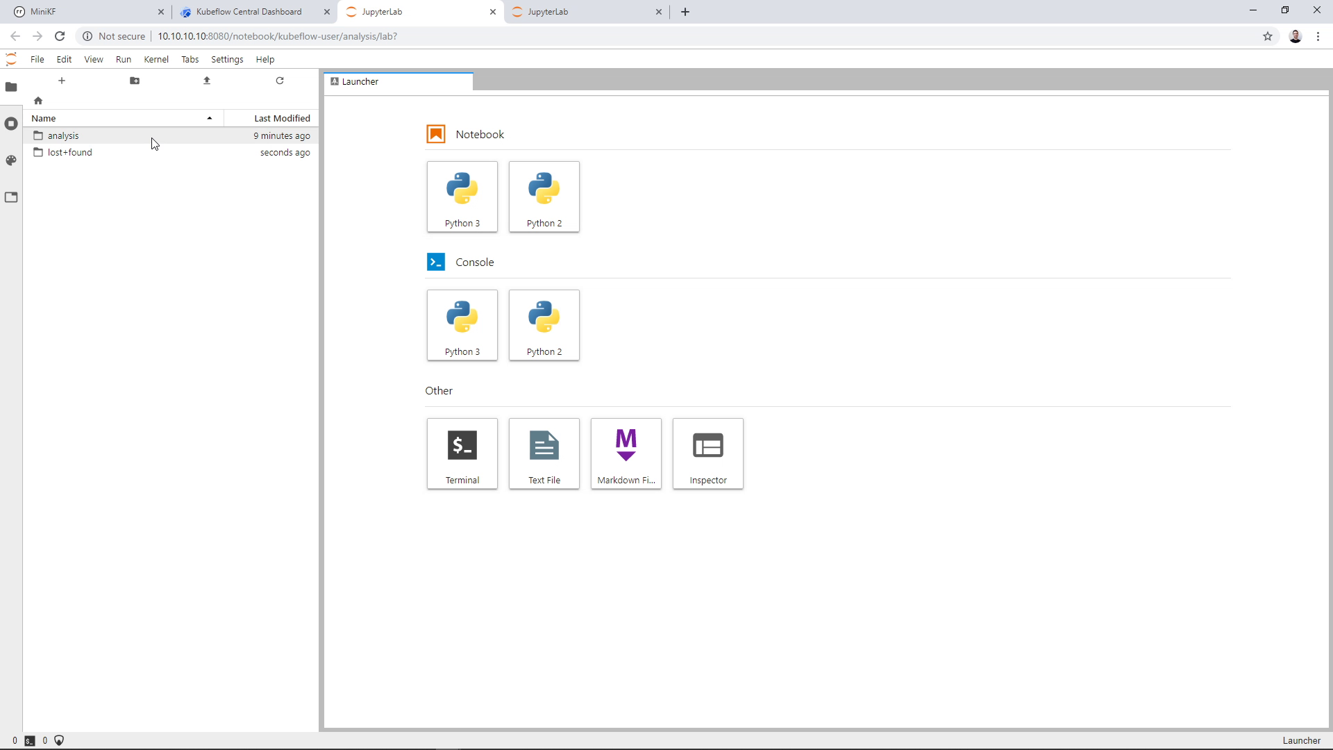
Inside the Notebook, you can see the Data Volume that we created by cloning the pipeline snapshot:
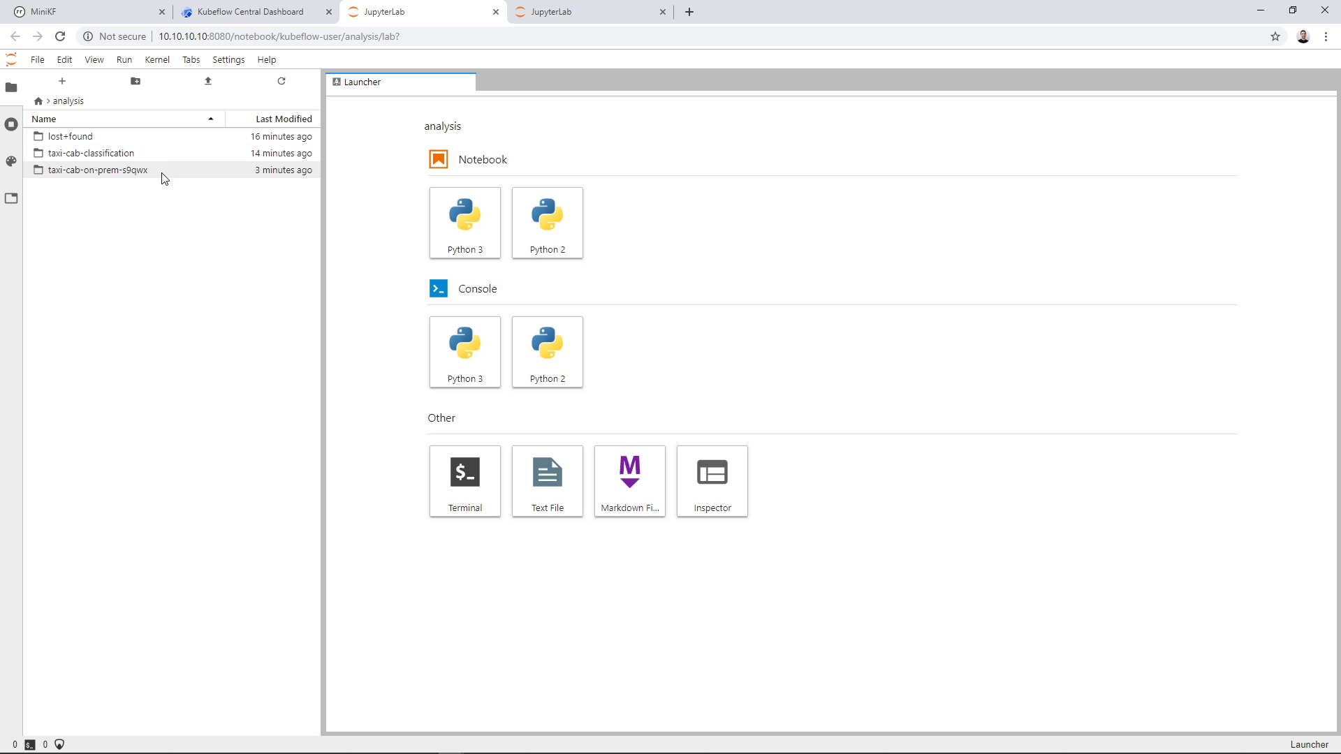
Inside the Data Volume you can see the input data of the pipeline “taxi-cab-classification”, and the output data of the pipeline “taxi-cab-classification-s9qwx”. Note that you will see a different alphanumerical sequence in your Notebook. Open the second folder to view the pipeline results:
You can see the results of every step of the pipeline:
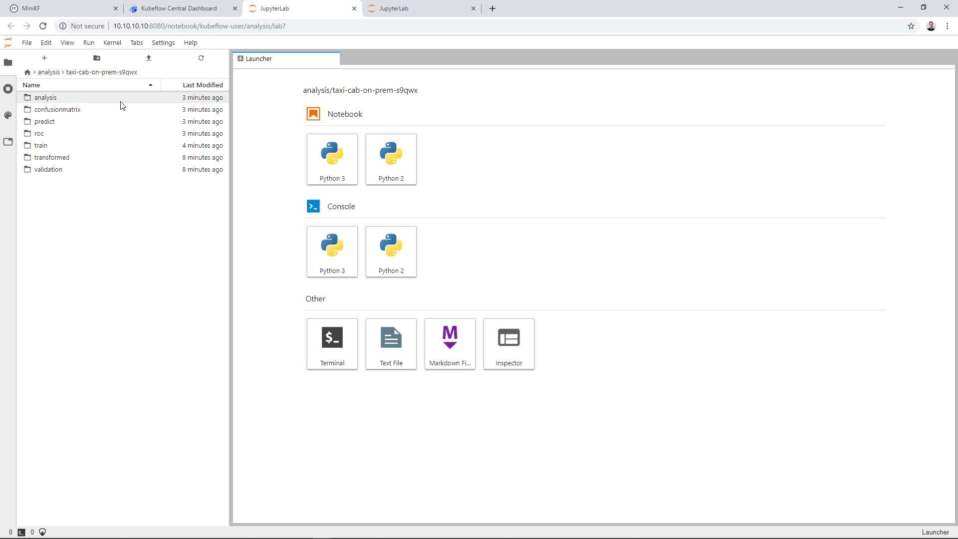
Let’s go inside the analysis folder to see how the model performed:
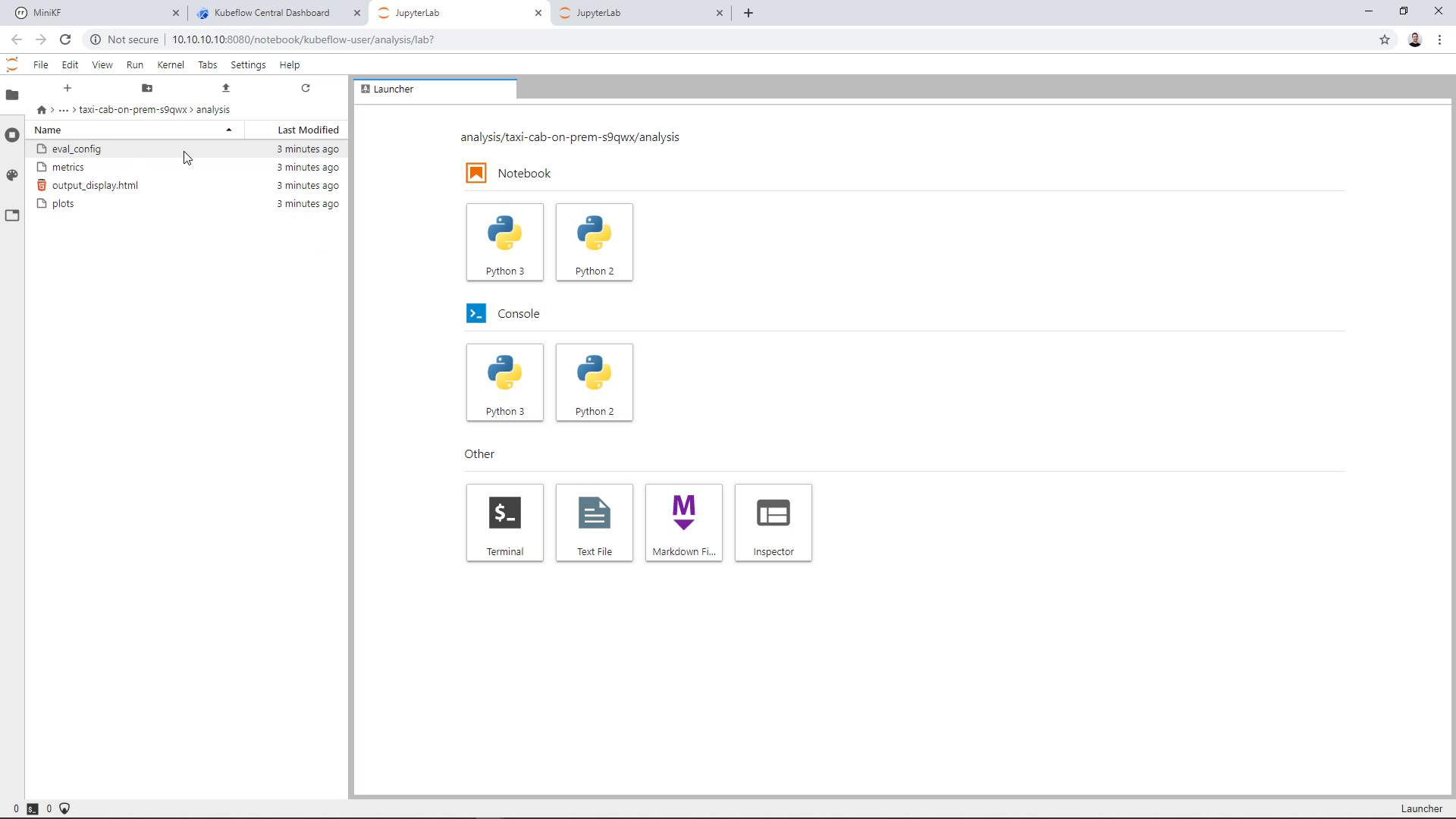
Open the “output_display.html” file:
Click on “Trust HTML” to be able to view the file:
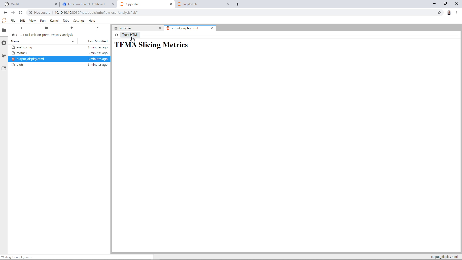
Here is how the model performed:
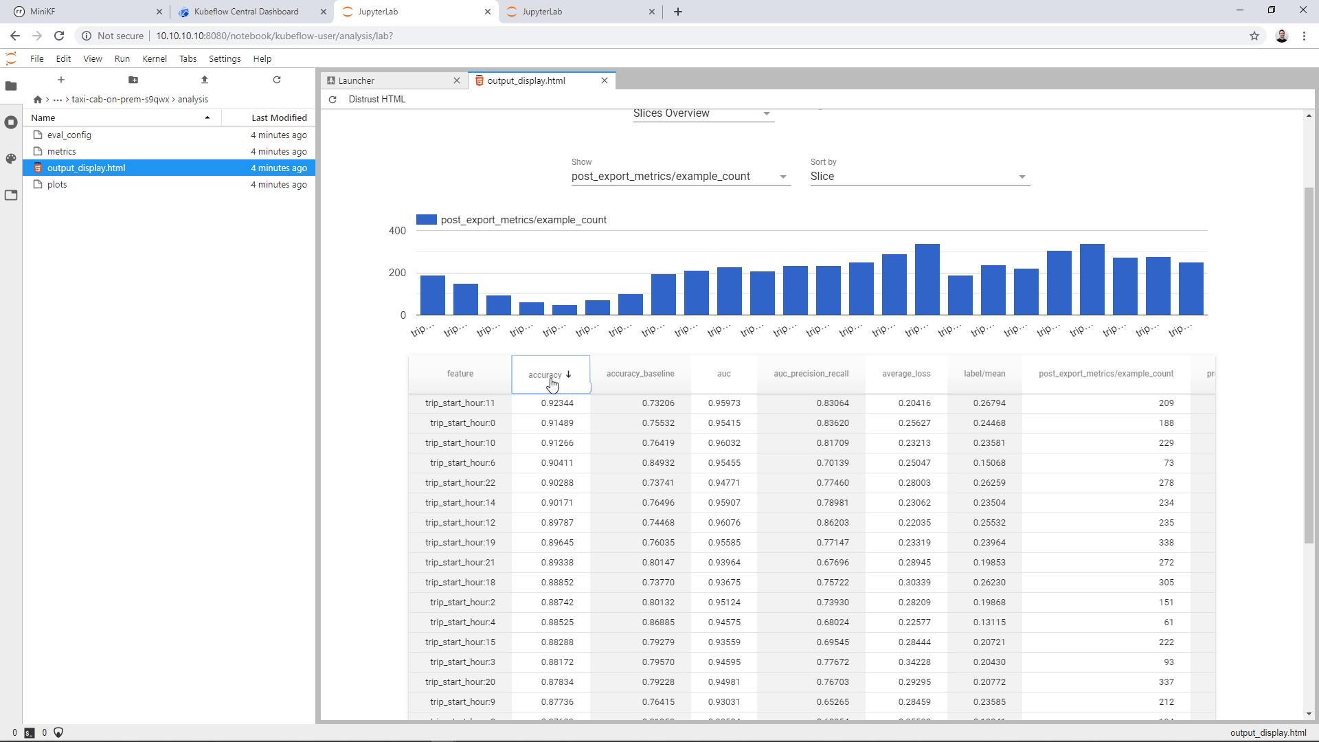
Note: this page is using HTML imports, a feature of the web components spec which is now deprecated. Most probably you won’t be able to view the model performance.
More MiniKF tutorials
- From Notebook to Kubeflow Pipelines with MiniKF & Kale
- Optimize a model using hyperparameter tuning with Kale, Katib, and Kubeflow Pipelines
Talk to us
Join the discussion on the #minikf Slack channel, ask questions, request features, and get support for MiniKF.
To join the Kubeflow Slack workspace, please request an invite.
Watch the tutorial video
You can also watch the video of this tutorial: