

Welcome to the latest installment of Arrikto’s ongoing series of blog posts that demonstrate how to take popular Kaggle competitions and convert them into Kubeflow Pipelines. All the converted Kaggle competitions in the series are contributed to the open source Kubeflow project for others to use and distribute. If you are interested in making a similar contribution, learn more.
Wait, What’s Kubeflow?
Kubeflow is an open source, cloud-native MLOps platform originally developed by Google that aims to provide all the tooling that both data scientists and machine learning engineers need to run workflows in production. Features include model development, training, serving, AutoML, monitoring and artifact management. The latest 1.5 release features contributions from Google, Arrikto, IBM, Twitter and Rakuten. Want to try it for yourself? You can get started in minutes with a free trial of Kubeflow as a Service, no credit card required.
About the House Prices – Advanced Regression Techniques Kaggle competition
Ask a home buyer to describe their dream house, and they probably won’t begin with the height of the basement ceiling or the proximity to an east-west railroad. But this playground competition’s dataset proves that much more influences price negotiations than the number of bedrooms or a white-picket fence.
With 79 explanatory variables describing nearly every aspect of residential homes located in Ames, Iowa, Kaggle’s House Prices competition challenges data scientists to predict the final price of each home.
In this blog, we will show how to run Kaggle’s House Prices – Advanced Regression Techniques Kaggle competition on Kubeflow using the Kubeflow Pipeline SDK and the Kale JupyterLab extension.
You can find the data, files and notebook for this example on GitHub here.
If you’d like to sit through an instructor-led workshop based on this Kaggle competition, you can register here.
Prerequisites for Building the Kubeflow Pipeline
Kubeflow
If you don’t already have Kubeflow up and running, we recommend signing up for a free trial of Kubeflow as a Service. It’s the fastest way to get Kubeflow deployed without having to have any special knowledge about Kubernetes or use a credit card.
To start building out the Kubeflow pipeline, you need to get yourself acquainted with the Kubeflow Pipelines documentation to understand what pipelines are, their components and what goes into these components. There are different ways to build out a pipeline component as mentioned here. In the following example, we are going to use lightweight Python functions based components for building the pipeline.
Building the Kubeflow Pipeline
Step 1: Installing the Kubeflow Pipeline SDK and Importing the Required kfp Packages to Run the Pipeline
Let’s get started by opening up the house-prices-kfp.ipynb notebook. Run the following commands.
You’ll need to uncomment the '!pip install' command if you haven’t yet installed Kubeflow Pipelines (kfp).
From kfp, we will be importing func_to_container_op which will help in building the pipeline tasks from the Python functions and we will use InputPath, plus OutputPath from the components package to pass paths of the files or models to these tasks. The passing of data is being implemented by kfp’s supported data passing mechanism. InputPath and OutputPath are how you pass on the data or model between the components.
Step 2: Building the Pipeline Components
Our Kubeflow pipeline is broken into five main components:
- Download data
- Load and preprocess data
- Create features
- Train data
- Evaluate data
The first pipeline component consists of downloading the data from GitHub URL. The GitHub URL is the download link for a zipped data file.
We are using the existing yaml file available from the Kubeflow Pipeline example for the creation of the pipeline task to download the data.
For loading the data from the zip file downloaded during the Download_data task, we need to get access to the file path of the zip which we do by specifying the InputPath parameter in the definition of the Python function.
The output obtained from the Download_data task is being passed on to the load_and_preprocess_data Python function through the InputPath.
For the Download_data task, we used the load_component_from_url method to create the pipeline task. In this step, we use func_to_container_op for the same.
In order to work with the data, certain packages have to be installed and imported for each pipeline component, and this needs to be done repeatedly if they are the same packages because each pipeline component is basically a container instance independent of the others.
func_to_container_op provides the packages_to_install argument to streamline this process. To keep track of the packages to be installed we define a common list of the packages which we pass on to each pipeline task except the Download_data task.
func_to_container_op also takes in base_image as an optional argument which by default is Python 3.7. If needed, a custom Docker image can also be passed on to the argument.
load_and_preprocess_data passes on two outputs to the next pipeline component function through OutputPath.
Since we have two outputs, we need to specify the name of the output while getting them as inputs.
The data passed to the featured_data_task are the training and test data in csv format. As of now, we can’t pass DataFrames directly through InputPath and OutputPath but we can pass them as artifacts through local or external storage. Note: there are ways to convert data into other formats which preserve the contents/information of the DataFrame, but this is an advanced topic and is outside of the scope of this tutorial.
We create the next pipeline components as we did for the load_and_preprocess_data task. The only changes we have are with the train_data and eval_data functions.
We pass on the trained ‘XGBoost’ model as an input to eval_data. For this we have to explicitly specify in the InputPath and OutputPath that a model is being passed, and we have to save and load the model using the XGBoost package. With csv file paths you don’t have to specify this information explicitly. You can refer to the documentation for more details on the specification of input and output parameter names.
Step 3 : Creating the Pipeline Function
After building all the pipeline components, we have to define a pipeline function that connects all the pipeline components with their appropriate inputs and outputs. This code, when run, will generate the pipeline graph.
Our pipeline function takes in the GitHub URL as an input to start with the first pipeline task, viz. download_data_task.
Step 4 : Running the Pipeline Using the kfp.Client Instance
There are different ways to run a pipeline function as mentioned in the documentation. In this tutorial, we will run the pipeline using the Kubeflow Pipelines SDK client.
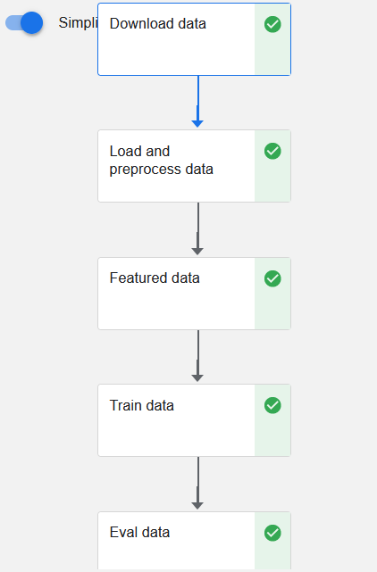
Once all the cells are executed successfully, you should see two hyperlinks, ‘Experiment details’ and ‘Run details’. Click on the ‘Run details’ link to observe the pipeline running.
The final pipeline graph will look as follows:
Is There an Easier Way to Create a Kubeflow Pipeline?
You bet! If you want to automate most of the steps illustrated in the previous example, then we recommend making use of the open source JupyterLab extension called Kale. Kale is built right into Kubeflow as a Service and provides a simple UI for defining Kubeflow Pipelines directly from your JupyterLab notebook, without the need to change a single line of code, build and push Docker images, create KFP components or write KFP DSL code to define the pipeline DAG. In this next example, we’ll show you just how easy it is.
Understanding Kale Tags
With Kale you annotate cells (which are logical groupings of code) inside your Jupyter Notebook with tags. These tags tell Kale how to interpret the code contained in the cell, what dependencies exist and what functionality is required to execute the cell.
Step 1: Annotate the Notebook with Kale tags
Kale tags give much better flexibility when it comes to converting a notebook to a Kubeflow pipeline.
For the Kaggle notebook example, we are using Arrikto’s MiniKF packaged distribution of Kubeflow. If you are using MiniKF then Kale comes preinstalled. For users with a different Kubeflow setup, you can refer to the GitHub link for installing the Kale JupyterLab extension on your setup.
The first step is to open up the Kale Deployment panel and click on the Enable switch button. Once you have it switched on, you should see the following information on the Kale Deployment panel.
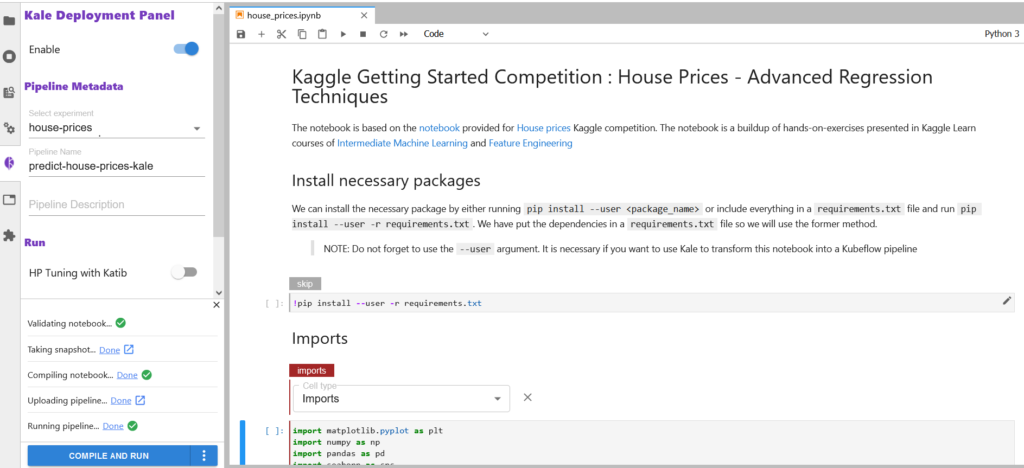
We already have “Select Experiment” and “Pipeline Name” selected. If you are starting fresh, you can create a new experiment by clicking on ‘New Experiment’ in the dropdown box and creating a new pipeline name for it.
Let’s start annotating the notebook with Kale tags.
There are six tags available for annotation:
- Imports
- Functions
- Pipeline Parameters
- Pipeline Metrics
- Pipeline Step
- Skip Cell
Our first annotation is for imports. First we will install all the required packages (not available under the standard python library) by using the requirements.txt file.

Once you have everything installed, annotate the cell with the “Skip Cell” tag as you don’t want to run this cell everytime you run the pipeline.
Next we tag the cell with the “Imports” annotation as shown below:
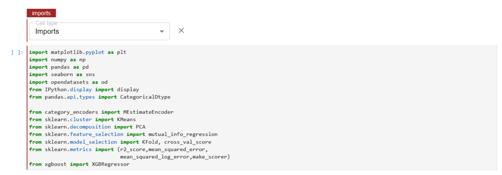
Once you have selected the “Imports” cell type, we see a red line highlight on the cell with the text Imports.
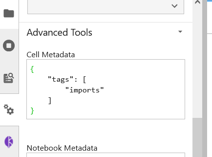
You can also see the tags being created by checking out the Cell Metadata by clicking on Property Inspector above the Kale Deployment Panel button.
For our pipeline components, we are gonna use the “Pipeline Step” tag annotation. Let’s tag the pipeline component load_and_preprocess_data.

In the tag annotation, you select the type of tag you are annotating with, and specify the step name. The step name would be shown as the name of the pipeline component in the runtime execution graph. The load_and_preprocess_data doesn’t depend on any previous pipeline step so we leave the dependencies field blank.
Let’s now look at the code and understand what we are doing here. First, we try to convert the .csv data files available under the /data directory to pandas DataFrame for further processing. Now this /data directory gets created in the local volume attached to the notebook. This is being automated by Kale as the first pipeline component in the pipeline graph where two volumes get mounted for the main and data directory.

After the df_train and df_test DataFrames are created, we concatenate them so that we can use a single DataFrame, df, for preprocessing and reform the splits for the next pipeline component.
For preprocessing, we are passing df as an input to different functions outside the cell. Kale provides us with a better way to organize this. We annotate those functions with the “Functions” annotation.
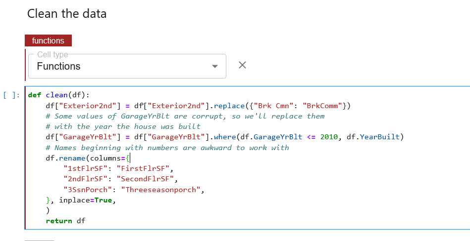
We can also do the same with other functions, but Kale provides the same tag annotation automatically for the next cells if the cell type is not otherwise specified, as shown below.
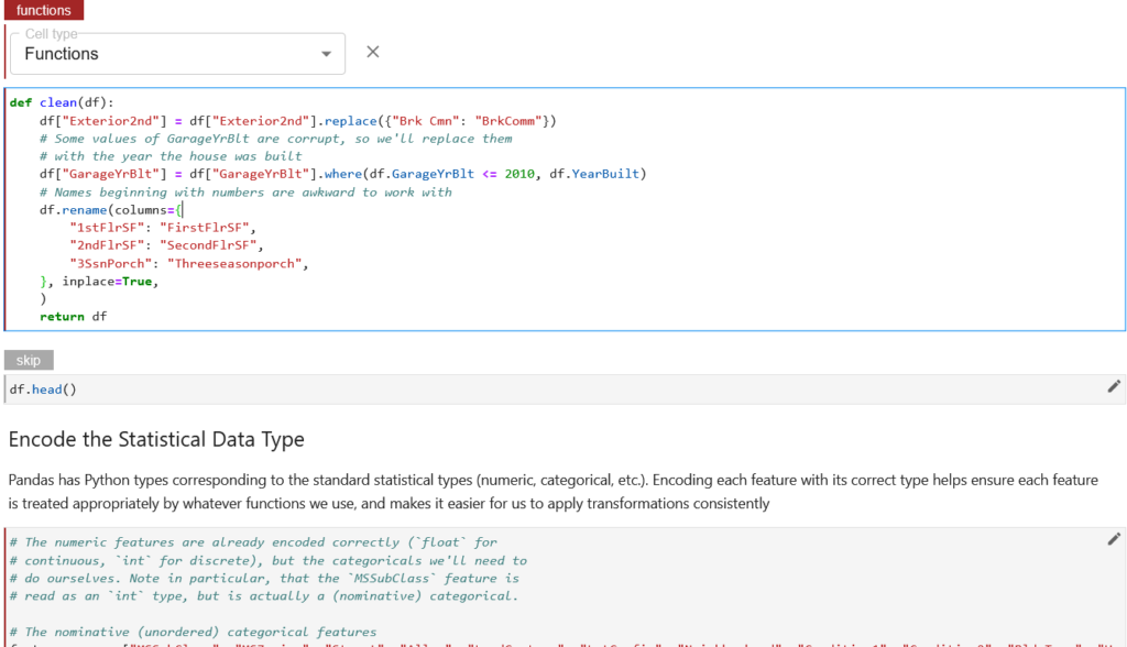
It can be observed from the above screenshot that the next cell has been highlighted with the same tag annotation without any specified tag annotation.
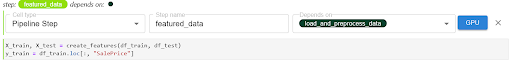
Now let’s move on to the next pipeline component. For the featured_data component, we are going to create and add features to the data. We are going to follow the same steps as we did for the load_and_preprocess_data component, but now this step depends on the output from the previous pipeline component.
For the train_data and eval_data pipeline components, we are going to follow the same steps as we did for the featured_data component.
Step 2: Run the Kubeflow Pipeline
Once you’ve tagged your notebook, click on the Compile and Run button in the Kale widget. Kale will perform the following tasks for you:
- Validate the notebook
- Take a snapshot
- Compile the notebook
- Upload the pipeline
- Run the pipeline
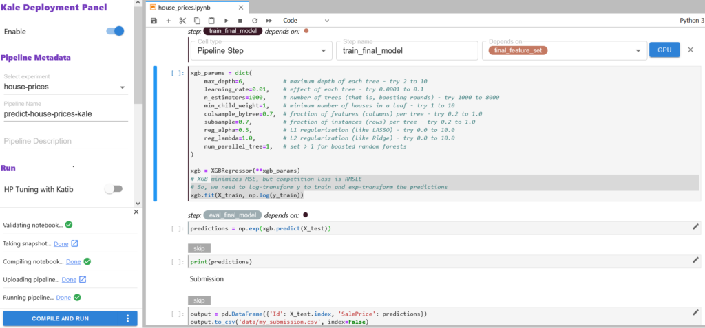
In the “Running pipeline” output, click on the View hyperlink. This will take you directly to the runtime execution graph where you can watch your pipeline execute and update in real time.
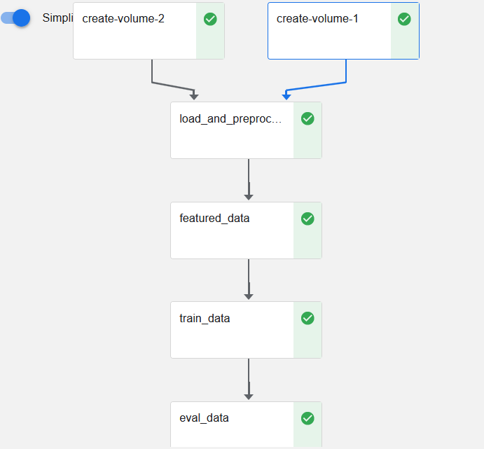
That’s it! You now have Kaggle’s House Prices competition running as a reproducible Kubeflow Pipeline with less coding and steps thanks to Kale.
By using Kale we eliminated several steps from the previous example:
- With the ‘vanilla’ version, you have to specify imports for each pipeline component again, be it a Docker image or a list of imports. Kale enables you to specify imports in one place, which is similar to what you do in a normal Juptyer notebook.
- In the “vanilla” Kubeflow Pipelines version, you have to manually pass the paths to the files and models required between components using
InputPathandOutputPath. Kale automates that by just specifying the dependencies with the pipeline steps, while annotating. - With the Kubeflow Pipelines version you have to pass on the csv version of the DataFrame, which loses all categorical information and has to reassign categories to the DataFrame. While there are alternative ways to transfer the data between components as an artifact through a local or external volume or using different data formats, doing so is an advanced topic that is outside the scope of this tutorial. Kale simply preserves the data structure and contents of the outputs.
- With the Kubeflow Pipelines version, you have to define the pipeline steps as inner functions to the pipeline component function. With Kale you can organize the pipeline steps using external functions with the help of the “Functions” tag annotation.
- Finally, Kale doesn’t require much learning and you can easily convert Kaggle notebooks to a Kubeflow pipeline, while with the ‘vanilla’ version there’s a bit of a learning curve involved.
What’s Next?
- Get started with Kubeflow in just minutes, for free. No credit card required!
- Get the code, data, and notebooks used in this example
- Try your hand at converting a Kaggle competition into a Kubeflow Pipeline