

Part 3 (of 3): The Dramatic Conclusion
Welcome to part three of the three-part series on using Kubeflow, Apache Spark, and Apache Mahout to denoise low-dose CT scans.
To recap to this point:
In March 2020 there was a large need for COVID rapid tests that could utilize existing hospital equipment (as opposed to having to be produced and distributed).
CT scans were known to be a good tool BUT among other things, they deliver high doses of radiation.
Low-dose CT scans, a technique that had been around for around 20 years, solved the radiation problem but they produce “noisy” images. A detailed exploration of this problem can be found in part two.
Through clever use of open source software and renting cloud time, we deliver a quickly and easily reproducible method for denoising low-dose CT scans. (Which we’ll discuss now.)
By open source software, I specifically mean how our heroes introduced in part one—Kubernetes, Kubeflow, Apache Spark, and Apache Mahout—will work together, overcome their differences, and solve this problem.
Getting CT Scans
So, we weren’t the only ones thinking along these lines at the time.
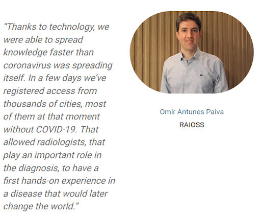
Dr. Paiva, a Brazilian radiologist, got CT scans of 10 patients with COVID from Wuhan, China and posted them to coronacases.org early in the pandemic to help other radiologists detect COVID with radiology (that is to show them “what it looks like”.)
The site is still up—you can go access coronavirus CT scans yourself right now. BUT for the purposes of this blog post series I recently tried updating code that I wrote in 2020 to ensure it still works (or at least know where it breaks), the metadata on the CT scans I was able to pull down are not standard. This process will still work on normal CT scans, which we’ll use instead. So you can go to coronacases.org and see what COVID looks like on a CT scan, and you can use this pipe to denoise CT scans, you just can’t denoise CT scans pulled from that site.
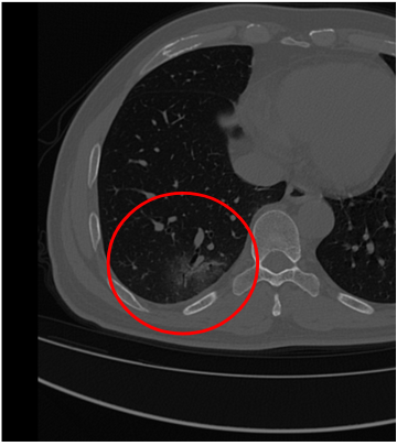
But, what does COVID look like in a CT scan?
First, let me state very clearly: I am not a radiologist, and I have no formal training in radiology.
But from the papers I’ve read, COVID in a thoracic CT scan presents as “Ground Glass Occlusions,” and I think that’s what we see in the image below.
A Pipeline to Make Dick Dale Jealous
So, big picture, what is going to happen here?
First, we collect images into an S3 bucket (we could use any storage device, but an S3 bucket was the easiest at the time).
Next we have a little Python app that reads DICOM images and converts them into numerical matrices (and writes them back to disk).
Next, we load the matrices into Spark as a resilient distributed data set (RDD).
Then, we wrap the RDD into Mahout distributed row matrices (DRM).
Then we do the distributed stochastic singular value decomposition (DS-SVD) on the DRM…
Which yields two new DRMs which we then write back to disk, and can then render images with various amounts of ‘denoising’ applied.
Step 1: Not Open Source
S3 buckets are a lingua franca in cloud object storage.
While I love using open source technologies and S3 is not open source, also important in our solution was the ability for others to pick up and use our pipe with minimal friction.
So the first step of our pipeline requisitions a persistent volume claim and then downloads the DICOM file from the S3 bucket to the PVC.
Other reasons I used S3: We’ll speak on it a bit more in a future paragraph, but the biggest reason was that I was using GCP’s compute engine which doesn’t support ReadWriteMany Persistent Volume Claims (RWX PVCs). We will need a disk that will support being written to by multiple sources simultaneously when we run our Spark job.
Note: S3 buckets aren’t performant. If you’re trying to do any real-world workloads, it would probably make sense to do some research here and find the optimal object storage for your use case.
Step 2: import answers
There’s an xkdc comic about a computer science undergrad handing in assignments in different languages, and for Python the professor says, “You can’t just import answers”.
That’s pretty applicable to this step. I needed to read DICOM images and of course there exists not one, but multiple libraries to do it. PyDICOM had the easiest on-ramp, so I used it.
When I was trying to recreate the pipe (read knock the dust off some two year old code), this was my first snag: the CT scans I pull from coronacases.org no longer have standard metadata. Someone who is good at hacking CT scans can probably figure it out, and I was able to read in a thoracic CT scan from another source, but just a warning: the CT scans at coronacases.org don’t work at the time of this writing.
To do the next bit of magic we need to convert a DICOM image into a numerical matrix. And PyDICOM makes that a pretty straight forward process. Like 15 lines of code straight forward.
So we read our DICOM file, process it into a numerical matrix, then dump the matrix into the PVC.
Now that’s the second time I’ve waved my hands and written to a PVC, but what is a PVC? A PVC is a PersistentVolumeClaim and is the more cloud native way to deal with data (as compared to an S3 bucket).
If you recall Kubernetes is just a layer that orchestrates a bunch of Docker containers, and a PVC gives you a volume you can mount to various containers, and as such you can treat it like some persistent disk space for handing large files off between containers, or more precisely, steps in our pipeline.
For instance, the first step was to requisition the PVC and download a DICOM image to it.
The next step (where we are now) was to process the DICOM file into a numerical matrix then write the matrix back to the PVC.
When I was doing this originally, back in 2020, I was using Kubernetes on GCP and the PVCs there are all “ReadWriteOnce” or RWO. That means they can only be mounted to one container at a time. So if I had like 30 executors, I’d have to take care of the replication myself, which wouldn’t be impossible, but was more effort than I was willing to put in.
NOTE: What access modes are available depends on your particular Kubernetes distribution. Rok (an Arrikto product) creates storage that is ReadWriteMany. For example, at the time of writing, PVCs in GCPs Kuberenetes distribution that are backed by ComputeEngine disks don’t support the RWX AcccessMode.
Step 3: Spark It Up!
Our next step will be to read that matrix into Apache Spark into an RDD.
If steps in our pipeline are just Docker containers, how then do we run a Spark job which might have a variable number of workers operating across multiple nodes?
In short it requires a ResourceOp; you define a ResourceOp with a manifest (like so many things in Kubernetes) AND in the manifest you specify how many workers you will use, and how big each worker can be. Now a clever trick here is you can define a manifest as a YAML (common) OR a JSON (uncommon, but legal) file, and the trick as you may see from the link is you can also define it as a ‘dict’ in Python.
This step is important and is what separates a real-world Spark job on Kubernetes from a proof of concept where you fool yourself into thinking something will scale which won’t.
You can kind of hack Spark into working with just a driver in one Docker container, but at that point, why are you using Spark? And while it might give you a word count, under any serious load it will blow up with an out of memory error.
Speaking of out of memory errors, if you thought error tracing on Spark was bad before, Spark jobs distributed on Kubernetes will be a special new layer of hell for you.
At the moment the errors I’m hitting have to do with the executors being disconnected from the driver. Probably some dumb config issue somewhere.
Also if you’re cribbing my code, be advised: the completion status is extremely hacky. There are much cleaner ways to exit now (again, there was a two year gap between writing the code and this blog).
Although this step involves running Spark in Kubernetes using Kubeflow, stay tuned for a future blog post all about Spark on MiniKF.
Step 4: Shoehorn Mahout in at Any Cost
Anyone who has followed me for any amount of time knows that I love to randomly insert Apache Mahout into things. This however is an instance where it is just the tool for the job!
Our matrix from the last step is in an RDD, also we’re running Apache Mahout on top of Spark, so we must wrap our RDD into a distributed row matrix or DRM.
This whole project really didn’t turn into the Mahout time to shine I had hoped. Mahout only accounts for about seven lines of code:
- One to wrap the RDD
- Three to get and set some parameters
- One to execute the ds-svd
- Three to write the output
Wait, what is SVD?
So allow me to do some hand waving here as getting into what a singular value decomposition (SVD) is and how it works is easily a week of lectures in a college level advanced linear algebra class. And then this isn’t even a full on SVD, but a distributed stochastic singular value decomposition (DS-SVD) which was the subject of a doctoral thesis by Nathan Halko, whom I owe a beer should I ever meet him because this technique has powered several of my talks now. So Dr. Halko, if you’re reading, first, thank you; and second, let’s get a beer.
So a singular value decomposition will take a matrix and spit out two other matrices and a vector. Here are some links to entire posts about what SVD is, if you care go read/watch/listen:
- Wikipedia (only useful if you already know what it is)
- MIT Lecture
- Blog post on Medium with a cool header image (but it’s on Medium so only go if you absolutely can’t find anything else).
What this denoising technique in essence boils down to is doing a principal component analysis (PCA) on an image and the idea is that the noise won’t be that important.
Now that is a gross oversimplification, but for us open source enthusiasts, it’s close enough given our time constraints. So we’re going to do a PCA and just trim off the ‘noise’ vectors at the end—too easy right?
A couple of side questions and answers:
Why not use NumPy? I tried using NumPy just to see what would happen and it estimated it would need 500GB of RAM to do a non-distributed non-stochastic singular value decomposition, which exceeds the specs of my desktop or anything I saw for rent in the cloud.
Why not use Spark’s built-in linear algebra package? Well, SparkML focuses more on machine learning and the SVD method is not distributed or stochastic, which will limit it to only running on one node, which gives us the same issue as NumPy.
So What?
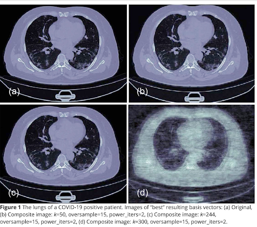
So here we see some results from the paper we published on this topic.
Let me be candid and say it is unclear, but unlikely, that the originals were low-dose CT scans. However, we can see how images degrade if we denoise them too much.
There is information in the paper about how we recombined them. The recombination is a straightforward matrix multiplication and could be easily done in a web browser with JavaScript, though, I think I used Python.
It’s a typical signal and noise problem. We are doing this method to remove noise, but we can see from (d) if you remove too much noise you also start to lose signal.
The End … ?
I hope you have been entertained (in my best Russel Crowe voice) by this three-part blog series recapping research that began in 2020. I spent all of part two setting up why we did all of this instead of just using rapid tests. Naturally, now at the time of this writing we know that rapid tests became cheaply and widely available, which is overall, a good thing.
But beyond entertainment, I hope this series has also been a good example of how to use Apache Spark in Kubeflow. (Hopefully better once I work out the kinks.) The code for all of this, can be found here.
Fun fact: The “how to” (this post) of this series is chapter 9 of an O’Reilly book some friends and I wrote on Kubeflow. That is how to actually build a pipeline for denoising CT scans.
Another fun fact: The “why” (part two) was published here in a peer reviewed journal. It digs more into the math and literature review of low-dose CT scans and denoising techniques. If you’re a radiologist who accidentally stumbled into this series, I’m sorry, I should have directed you there at the outset. It also shows I didn’t skip over the math because I didn’t know it, but because it has been covered in better detail elsewhere.
Final Thought
Like Jerry Springer, I would like to close out a longer form piece like this with some pseudo-wise recap.
It’s easy to look back with the benefit of hindsight and think ‘oh that was a silly thing to do’ (applicable to this series, the person in part two wearing the cootie shield, and the best of us the morning after a wild party). But in the moment everyone is doing the best they can, and open source software helps facilitate that. So I hope you can find some time in your busy week to show some gratitude to the contributors on your favorite projects; it could be as simple as getting on their mailing list and sending a “thanks for everything you do email”. It might feel like you’re just making noise, but it is appreciated.
Until next time, take care of yourself…and each other.